TODO
- Update commentary to be more intensive
- Finish hyperparameter tuning
- Add note on overfitting with random forests & gradient boosted trees
Ensemble Methods
One quote I heard in the beginning of my machine learning journey is "if you don't have a favorite algorithm yet, pick the random forest". I'm glad that I heard that early on, because it has proven itself multiple times along with the other algorithms in the ensemble family.
There are a few good reasons why ensemble methods are my favorite family of models. Not only are they often extremely powerful in predictive performance (often topping the leaderboards on Kaggle competitions for structured data), but they still maintain some semblance of interpretability and can often be parallelized to utilize all cores of a CPU.
I recently gave a talk on ensemble methods. at a local meetup group, and this is a more flushed out version of the hands-on portion that includes a more difficult dataset and more complete hyperparameter tuning.
Overview
In this post, we'll train a few ensemble models on an artificial dataset for binary classification. We'll use scikit-learn to compare a few different types of ensemble methods, and then use XGBoost and LightGBM for more specialized implementations of gradient boosting. Additionally, we'll go over hyperparameter tuning and discuss a few strategies for tuning ensemble models.
Setup
The setup here is largely a series of import statements, creating an artificial classification dataset with scikit-learn's make_classification function, and then creating a function to train our models and gather various metrics.
import sys
import time
import scipy
import numpy as np
import pandas as pd
import matplotlib.pyplot as plt
import seaborn as sns

from sklearn import datasets
from sklearn.model_selection import train_test_split
from sklearn.model_selection import RandomizedSearchCV
from sklearn import ensemble
from sklearn import linear_model
from sklearn import metrics

print(time.strftime('%Y/%m/%d %H:%M'))
print('OS:', sys.platform)
print('Python:', sys.version)
print('NumPy:', np.__version__)
print('Pandas:', pd.__version__)

%matplotlib inline
2018/07/11 19:39
OS: win32
Python: 3.5.5 | packaged by conda-forge | (default, Apr  6 2018, 16:03:44) [MSC v.1900 64 bit (AMD64)]
NumPy: 1.12.1
Pandas: 0.23.1
Creating an artificial data set with scikit-learn's make_classification function.
TODO: Increase the size of the dataset and re-run
# Creating an artificial dataset to test algorithms on
data = datasets.make_classification(#n_samples=300000,
            n_samples=3000,
                                    n_classes=2,
                                    n_features=30,
                                    n_informative=10,
                                    n_redundant=5,  # Superfluous features working as noise for the algorithms
                                    flip_y=0.5,  # Introduces additional noise
                                    class_sep=0.7,
                                    n_clusters_per_class=10,
                                    random_state=46)

# Assigning features/labels to variables for ease of use
X = data[0]  # Features
y = data[1]  # Label

# Train/test split
X_train, X_test, y_train, y_test = train_test_split(X, y, test_size=0.30, random_state=46)

# Putting into a dataframe for viewing
df = pd.DataFrame(X)
df['label'] = y

df.head()
| 0 | 1 | 2 | 3 | 4 | 5 | 6 | 7 | 8 | 9 | ... | 21 | 22 | 23 | 24 | 25 | 26 | 27 | 28 | 29 | label | |
|---|---|---|---|---|---|---|---|---|---|---|---|---|---|---|---|---|---|---|---|---|---|
| 0 | -2.099007 | 0.787135 | -0.686102 | -1.228830 | 0.723556 | -0.311079 | -0.952826 | 0.867668 | -1.642571 | 0.624871 | ... | 0.987041 | -0.377789 | 0.242981 | -0.792679 | -1.715772 | -0.420792 | -1.729152 | 1.308256 | -0.700561 | 1 |
| 1 | -0.801402 | -3.851769 | 1.538805 | 0.565783 | 0.526172 | 0.752565 | 0.014558 | -0.240075 | -1.479138 | 1.819075 | ... | -0.153594 | -0.324068 | -2.060220 | 1.541481 | 1.297861 | -1.228942 | 0.494606 | 2.167953 | 0.178436 | 1 |
| 2 | -5.662407 | -5.853161 | 1.625716 | -0.390593 | 1.199284 | 1.888906 | -1.019720 | -1.392650 | 3.012919 | -1.139037 | ... | -0.335733 | -0.468439 | -1.996023 | 2.419778 | -1.558457 | -0.539612 | -1.159566 | 3.362889 | -0.891273 | 0 |
| 3 | 1.569256 | 5.984285 | -1.678201 | -0.601325 | 0.470834 | 0.688409 | -2.392620 | -0.946743 | -2.713660 | 1.422514 | ... | -0.161714 | -1.189745 | -0.837363 | -0.825927 | -1.654660 | -0.339540 | 1.216920 | 0.145422 | 1.459836 | 1 |
| 4 | 2.881864 | 5.945795 | -1.627379 | -1.361672 | -0.773137 | -0.071754 | -4.075099 | 1.901061 | -4.294425 | 0.795730 | ... | 0.656566 | -0.235963 | -2.146111 | 0.594049 | 2.290443 | 0.330266 | -0.019847 | -5.770743 | 0.815581 | 1 |
5 rows × 31 columns
In order to adhere to DRY typing, we'll create a function to train our models and gather the accuracy, AUC, log loss, and model training time.
# Data frame for gathering results
results = pd.DataFrame(columns=['Accuracy', 'LogLoss', 'AUC', 'TrainingTime'])
tuned_results = pd.DataFrame(columns=['Accuracy', 'LogLoss', 'AUC', 'TrainingTime', 'NumIterations'])

# Function for training a model and retrieving the results
def train_model_get_results(model, model_name):
    '''
    Trains a model and appends the results to the results dataframe

    Input:
        - model: The model with specified hyperparameters to be trained
        - model_name: The name of the model to be used as the index
        - is_tuned: A binary flag for if hyperparameter tuning has been performed

    Output: The results dataframe with the model results added

    Note: Only works with scikit-learn models and frameworks that integrate
          with the scikit-learn API
    '''

    # Collecting training time for results
    start_time = time.time()

    print('Training the model')
    model.fit(X_train, y_train)

    end_time = time.time()
    total_training_time = end_time - start_time
    print('Completed')

    # Calculating the testing set accuracy with the score method
    accuracy = model.score(X_test, y_test)

    # Calcuating the AUC and log loss with predicted probabilities
    class_probabilities = model.predict_proba(X_test)
    log_loss = metrics.log_loss(y_test, class_probabilities)
    auc = metrics.roc_auc_score(y_test, class_probabilities[:, 1])

    # Adding the model results to the results dataframe
    model_results = [accuracy, log_loss, auc, total_training_time]
    results.loc[model_name] = model_results

    print('\n', 'Non-tuned results:')
    return results
Baseline
It's always useful to have a baseline to compare against and let us know generally how difficult a problem is going to be. I like to use linear or logistic regression due to each them being extremely fast to train.
# Instantiating the model
logistic_regression = linear_model.LogisticRegression()

# Using our user defined function to train the model and return the results
train_model_get_results(model=logistic_regression, model_name='Logistic Regression')
Training the model
Completed

 Non-tuned results:
| Accuracy | LogLoss | AUC | TrainingTime | |
|---|---|---|---|---|
| Logistic Regression | 0.505556 | 0.697955 | 0.491237 | 0.015628 |
Bagging
Bagging (bootstrap aggregating) is the technique that aggregates models built with bootstrapping, or sampling with replacement, via a majority vote or by averaging the predictions. The trees are independent of each other and can be built in parallel.
Bagging models tend to decrease variance.
Random Forest
The most popular bagging algorithm is the random forest. This algorithm works by building a series of decision trees where each tree uses a random selection of variables, and then decision trees vote on the final answer.
More specifically, for each tree:
- Use a different training sample with replacement (bootstrapping) for the data
- For each node, choose a number of random attributes and find the best split
- Typically is not pruned in order to have a smaller bias
Once these trees are grown, a majority vote among all of the trees will be used to make predictions.
The main ideas here are that the randomness makes a set of diverse models that helps improve accuracy and using random subsets of features to consider at each split helps make it more efficient to train.

Advantages:
- Robustness against over-fitting
- Since the model is created through dense randomness, the generalization is typically better, and you can usually increase the accuracy with the number of trees up until a saturation point
- Able to parallelize training multiple trees at once and thus speed up training time
random_forest = ensemble.RandomForestClassifier(n_jobs=-1)  # n_jobs=-1 uses all available cores

train_model_get_results(random_forest, model_name='Random Forest')
Training the model
Completed

 Non-tuned results:
| Accuracy | LogLoss | AUC | TrainingTime | |
|---|---|---|---|---|
| Logistic Regression | 0.505556 | 0.697955 | 0.491237 | 0.015628 |
| Random Forest | 0.523333 | 0.810627 | 0.532343 | 0.171863 |
Boosting
Boosting methods train a sequence of weak learners (a learner that is barely better than random chance) where each successive model focuses on the parts that the previous model got wrong. The trees have to be built in a sequence and generally cannot be built in parallel without clever tricks.
Boosting models tend to decrease bias.
Gradient Boosting
While there are a few different boosting algorithms, gradient boosting is arguably the most popular. It's main differentiation from the others is that it uses gradient descent to decide what to focus on in order to minimize loss for the new trees being built in the sequence. This typically gives it performance advantages over other boosting algorithms.
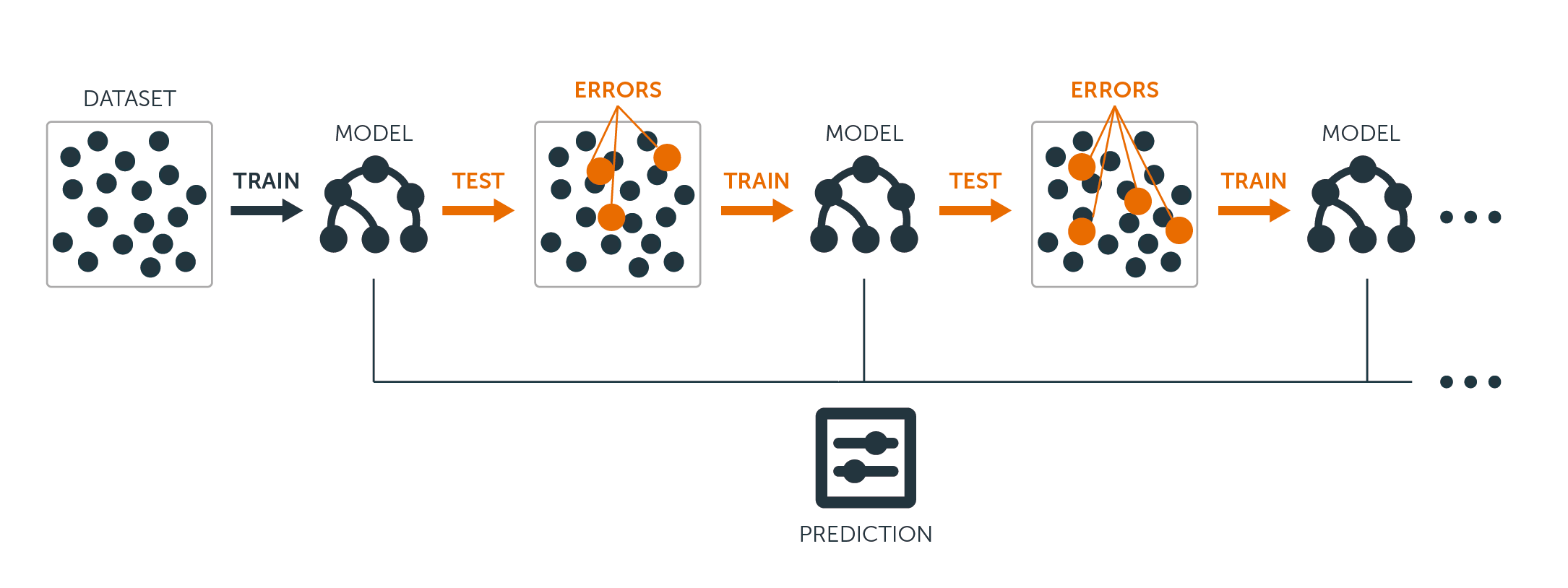
Source: BigML
Advantages:
- Can often outperform random forests when properly tuned
Disadvantages:
- Typically overfits easier than bagging
- Sensitive to noise & extreme values
- Has to be built sequentially, so cannot parallelize without tricks
gradient_boosting = ensemble.GradientBoostingClassifier()

train_model_get_results(gradient_boosting, model_name='Gradient Boosted Trees')
Training the model
Completed

 Non-tuned results:
| Accuracy | LogLoss | AUC | TrainingTime | |
|---|---|---|---|---|
| Logistic Regression | 0.505556 | 0.697955 | 0.491237 | 0.015628 |
| Random Forest | 0.523333 | 0.810627 | 0.532343 | 0.171863 |
| Gradient Boosted Trees | 0.546667 | 0.693403 | 0.561060 | 1.031190 |
Note on interpretability
It's possible to obtain "feature importance" from both bagging and boosting methods. These are not as interpretable as coefficients from linear/logistic regressions, but can still give us an idea of what is happening.
Note that the multicollinearity assumption applies here - these interpretations will be misleading if the features are heavily correlated with each other.
def feature_importance(model):
    '''
    Plots the feature importance for an ensemble model from scikit-learn
    '''
    feature_importance = model.feature_importances_
    feature_importance = 100.0 * (feature_importance / feature_importance.max())
    sorted_idx = np.argsort(feature_importance)
    pos = np.arange(sorted_idx.shape[0]) + .5
    plt.figure(figsize=(15, 8))
    plt.subplot(1, 2, 2)
    plt.barh(pos, feature_importance[sorted_idx], align='center')
    plt.yticks(pos, sorted_idx)
    plt.xlabel('Relative Importance')
    plt.title('Variable Importance')
    plt.show()


feature_importance(gradient_boosting)
Stacking
Stacking is the final ensemble technique where we combine several different models into a chain of sorts. It is structured similarly to a neural network where layers of models provide predictions that the next layer then uses as inputs. Ultimately, the meta-classifier creates a final prediction.
This is a little more nuanced than blending models (averaging their predictions for a final prediction) as the meta-learner learns how useful each of the models are.
Advantages:
- Can be more performant when properly tuned
Disadvantages:
- Much more computationally costly
- More difficult to tune
- Complete loss of interpretability
We'll need another function that is similar to our previous one for training the models and getting the results. In this case, we'll deal with one layer of classifiers and use a logistic regression for the meta-learner. We'll use five different algorithms for the first layer, but this function is designed to accept any number of models.
def train_stacking_get_results(list_of_models):
    '''
    Trains a stacking classifier and appends the results to the rsults dataframe

    Input: list_of_models: a list of untrained scikit-learn models

    Output: The results dataframe with the model results added

    Note: Only works with scikit-learn models and frameworks that integrate
          with the scikit-learn API
    '''
    # The meta learner is the one that takes the outputs from
    # the other models as input before final classification
    meta_learner = linear_model.LogisticRegression()

    # Collecting training time for results
    start_time = time.time()
    print('Training the model')

    # Fitting the first layer models
    for model in list_of_models:
        model.fit(X_train, y_train)

    # Collecting the predictions from the models for training
    model_output = []

    for model in list_of_models:
        class_probabilities = model.predict_proba(X_train)[:, 1]
        model_output.append(class_probabilities)

    # Re-shaping before passing to the meta learner
    X_train_meta = np.array(model_output).transpose()

    # Fitting the meta learner
    meta_learner.fit(X_train_meta, y_train)

    end_time = time.time()
    total_time = end_time - start_time
    print('Completed')

    # Collecting the predictions from the models for testing
    model_output = []

    for model in list_of_models:
        class_probabilities = model.predict_proba(X_test)[:, 1]
        model_output.append(class_probabilities)

    # Re-shaping before passing to the meta learner
    X_test_meta = np.array(model_output).transpose()

    # Collecting the accuracy from the meta learner
    accuracy = meta_learner.score(X_test_meta, y_test)

    # Calcuating the log loss with predicted probabilities
    class_probabilities = meta_learner.predict_proba(X_test_meta)
    log_loss = metrics.log_loss(y_test, class_probabilities)
    auc = metrics.roc_auc_score(y_test, class_probabilities[:, 1])

    # Printing coefficients of models
    print()
    print('Coefficients for models')
    for i, coef in enumerate(meta_learner.coef_[0]):
        print('Model {0}: {1}'.format( i+1, coef))

    model_results = [accuracy, log_loss, auc, total_time]
    results.loc['Stacking'] = model_results

    return results


# Adding extra imports for additional models
from sklearn import neighbors

# Defining the learners for the first layer
model_1 = linear_model.LogisticRegression()
model_2 = ensemble.RandomForestClassifier(n_jobs=-1)
model_3 = ensemble.RandomForestClassifier(n_jobs=-1)
model_4 = ensemble.GradientBoostingClassifier()
model_5 = neighbors.KNeighborsClassifier(n_jobs=-1)

# Putting the models in a list to iterate through in the function
models = [model_1, model_2, model_3, model_4, model_5]

# Running our function to build a stacking model
train_stacking_get_results(models)
Training the model
Completed

Coefficients for models
Model 1: -2.9603327700929984
Model 2: 6.827364713943086
Model 3: 6.967087517500586
Model 4: 0.7215877036971426
Model 5: 0.49496178638295857
| Accuracy | LogLoss | AUC | TrainingTime | |
|---|---|---|---|---|
| Logistic Regression | 0.505556 | 0.697955 | 0.491237 | 0.015628 |
| Random Forest | 0.523333 | 0.810627 | 0.532343 | 0.171863 |
| Gradient Boosted Trees | 0.546667 | 0.693403 | 0.561060 | 1.031190 |
| Stacking | 0.520000 | 0.994001 | 0.533464 | 1.593773 |
Hyperparameter Tuning
There two main methodologies for hyperparameter tuning:
- Manually testing hypotheses on how changing certain hyperparameters will impact the performance of the model
- Automatically checking a bunch of different combinations of hyperparameters using either a grid search or a randomized search
For this post, we will discuss a few strategies for the first option, and then go with the second option by using a randomized search.
Between grid search and random search, grid search generally makes more intuitive sense. However, research from James Bergstra and Yoshua Bengio have shown that random search tends to converge to good hyperparameters faster than grid search. Here's a graphic from their paper that gives an intuitive example of how random search can potentially cover more ground when there are hyperparameters that aren't as important:
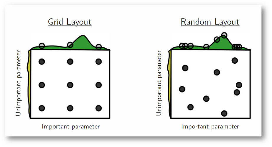
Source: James Bergstra & Yoshua Bengio
Hyperparameters & Decision Tree Structure
Because both random forests and gradient boosted trees use decision trees for their underlying structures, their hyperparameters are largely the same. Here's a recap of the decision tree structure and a quick summary of what each of the hyperparameters we'll be tuning are:

Source: Murtuza Morbiwala
Hyperparameters
This is list is not all-inclusive, but has most of the common hyperparameters:
- Number of Estimators: The number of decision trees to be trained
- A higher number typically means better predictions (at the cost of computational power) up until a saturation point where the model begins to overfit
- Max Depth: How deep a tree can be
- This should ideally be low for gradient boosting and large (or none) for random forests
- Minimum Samples per Split: The minimum samples considered to split a node
- A higher number typically results in better performance at the cost of computational efficiency
- Minimum Samples per Leaf: The minimum number of samples required to be a leaf node
- A lower number could potentially result in more noise being captured
- Max Features: The number of features to consider when looking for the best split
- A lower number typically reduces variance/increases bias and improves computational efficiency
- Max Leaf Nodes: The maximum number of leaf nodes for the tree
- A smaller number could help prevent overfitting
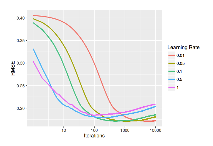
- Learning Rate (gradient boosting only): The adjustment/step size for each iteration
- A larger step size can help get better performance in fewer iterations, but will plateau at a lower performance
- A smaller step size will require more iterations (number of estimators) but will ultimately achieve a better performance
Here is an illustration on what a learning rate is and how too small or large of a learning rate can have adverse impacts:
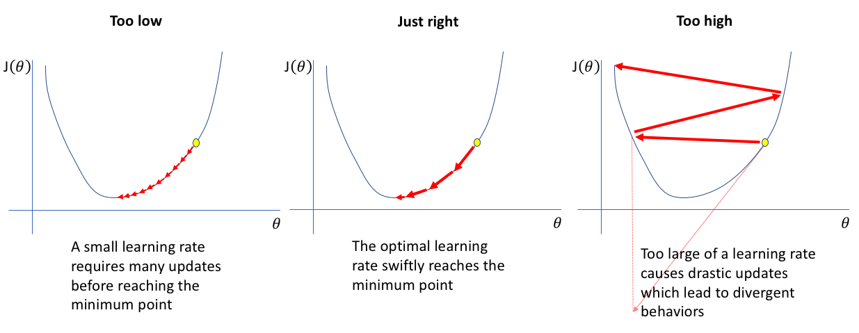 *Source: [Jeremy Jordan](https://www.jeremyjordan.me/nn-learning-rate/)*
Here is a more visual version of these hyperparameters on a tree:
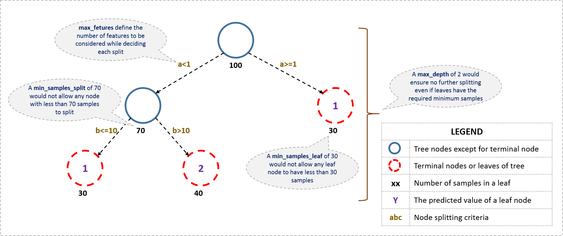 *Source: [Analytics Vidhya](https://www.analyticsvidhya.com/blog/2016/02/complete-guide-parameter-tuning-gradient-boosting-gbm-python/)*
General Strategies
Most strategies are specific to either random forests or gradient boosting, but there are a few strategies that apply to both.
- Increase the number of estimators until either just before overfitting begins to start occurring or there are severely diminishing returns in performance
- Compare the performance against the default parameters to see if this helps and how much
- Further adjust the model complexity (starting with tree depth)
- Decrease the complexity of the trees if you suspect the model is suffering from high variance
- Increase the complexity of the trees if you suspect the model is suffering from high bias
Remember that hyperparameter tuning is all about controlling model complexity in order to achieve the optimal state in the bias-variance tradeoff:
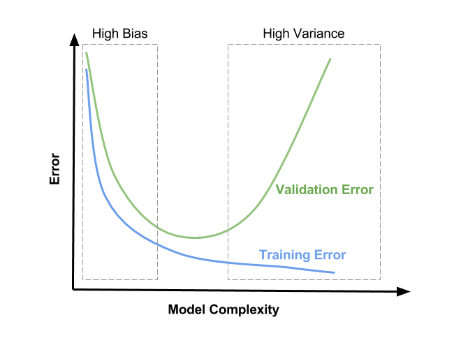 *Source: [Satya Mallick](https://www.learnopencv.com/bias-variance-tradeoff-in-machine-learning/)*
Setup
In order to do the actual hyperparameter tuning we need to create our third and final function. This will take a model, a dictionary of parameters, perform a random search for the number of iterations, and then give us our results.
def hyperparameter_tune_get_results(model, parameters, model_name, num_rounds=30):
    '''
    Performs a random search to find optimal hyperparameters and append the results
    to the tuned_results dataframe

    Input:
        - model: A scikit-learn model
        - parameters: A dictionary of parameters for the model
        - model_name: A string of the model name for the tuned_results dataframe
        - num_rounds: The number of rounds to try different hyperparameters

    Output: The tuned_results dataframe with the results appended
    '''

    # Reporting the default parameters before tuning
    print('Default Parameters:', '\n')
    print(model, '\n')

    # Defining the random search cross validation
    random_search = RandomizedSearchCV(model,
                                       param_distributions=parameters,
                                       n_iter=num_rounds, n_jobs=-1, cv=3,
                                       return_train_score=True, random_state=46,
                                       verbose=10)  # Set to 20 to print the status of each completed fit

    print('Beginning hyperparameter tuning')
    start_time = time.time()
    random_search.fit(X_train, y_train)
    end_time = time.time()
    total_training_time = end_time - start_time
    print('Completed')

    # Calculating the testing set accuracy on the best estimator with the score method
    accuracy = random_search.best_estimator_.score(X_test, y_test)

    # Calcuating the log loss with predicted probabilities
    class_probabilities = random_search.best_estimator_.predict_proba(X_test)
    log_loss = metrics.log_loss(y_test, class_probabilities)
    auc = metrics.roc_auc_score(y_test, class_probabilities[:, 1])

    # Adding the model results to the results dataframe
    model_results = [accuracy, log_loss, auc, total_training_time, num_rounds]
    tuned_results.loc[model_name] = model_results

    # Plotting the mean training accuracy from the different iterations
    sns.distplot(random_search.cv_results_['mean_test_score'])
    plt.title('Mean test score')

    print('Best estimator:', '\n')
    print(random_search.best_estimator_)

    print()
    print('Accuracy before tuning:', results.loc[model_name]['Accuracy'])
    print('Accuracy after tuning:', tuned_results.loc[model_name]['Accuracy'])

    print('\n', 'Tuned results:')
    return tuned_results
Baseline
For our logistic regression model, we're just going to tune the regularization parameter. One of the advantages of simpler models like this is that they are easier to tune because we don't have nearly as many hyperparameters to worry about.
Note: The number of rounds is being kept small in these examples to keep within time limits for the talk, but increase them in a real-world scenario for more effective hyperparameter tuning
parameters = {'C': scipy.stats.uniform(0, 10),  # Uniform distribution between 0 and 10
              'penalty': ['l1', 'l2']
             }

hyperparameter_tune_get_results(model=logistic_regression, parameters=parameters,
                                model_name='Logistic Regression', num_rounds=10)
Default Parameters:

LogisticRegression(C=1.0, class_weight=None, dual=False, fit_intercept=True,
          intercept_scaling=1, max_iter=100, multi_class='ovr', n_jobs=1,
          penalty='l2', random_state=None, solver='liblinear', tol=0.0001,
          verbose=0, warm_start=False)

Beginning hyperparameter tuning
Fitting 3 folds for each of 10 candidates, totalling 30 fits
[Parallel(n_jobs=-1)]: Done   5 tasks      | elapsed:    7.0s
[Parallel(n_jobs=-1)]: Done  10 tasks      | elapsed:    7.1s
[Parallel(n_jobs=-1)]: Done  17 tasks      | elapsed:    7.3s
[Parallel(n_jobs=-1)]: Done  27 out of  30 | elapsed:    7.8s remaining:    0.8s
[Parallel(n_jobs=-1)]: Done  30 out of  30 | elapsed:    7.9s finished
Completed
Best estimator:

LogisticRegression(C=6.8421729839625272, class_weight=None, dual=False,
          fit_intercept=True, intercept_scaling=1, max_iter=100,
          multi_class='ovr', n_jobs=1, penalty='l2', random_state=None,
          solver='liblinear', tol=0.0001, verbose=0, warm_start=False)

Accuracy before tuning: 0.505555555556
Accuracy after tuning: 0.505555555556

 Tuned results:
| Accuracy | LogLoss | AUC | TrainingTime | NumIterations | |
|---|---|---|---|---|---|
| Logistic Regression | 0.505556 | 0.697967 | 0.491222 | 8.296371 | 10.0 |

Random Forests
Because random forests are generally robust to overfitting and there aren't as many parameters to control as there are in gradient boosting, our hyperparameter tuning strategy doesn't have to be as nuanced.
I've found that increasing the number of trees has the most direct impact on performance. Because the saturation point of overfitting by too many trees is relatively high for random forests, we can usually increase them until our models take too long to train or there isn't much of a performance gain from using more trees. Scikit-learn's random forest implementation only uses 10 by default, but R's randomForest package uses 500 by default.
That's the first level of complexity to control, so after that it's looking into controlling the max depth for overall model complexity. How this is adjusted depends on if we need to reduce bias or variance.
We can also control a few other components like the number of features considered for each split or the minimum samples required for each split/leaf, but these may not have as large of an impact as the number of estimators or max depth.
# Creating the dictionary of parameters to use in the search
parameters = {'n_estimators': scipy.stats.randint(low=10, high=1000),  # Uniform distribution
              'max_depth': [None, 10, 30],  # Maximum number of levels in a tree
              'max_features': ['auto', 'log2', None],  # Number of features to consider at each split
              'min_samples_split': [2, 5, 10],  # Minimum number of samples required to split a node
              'min_samples_leaf': [1, 2, 4]  # Minimum number of samples required at each leaf node
             }

hyperparameter_tune_get_results(random_forest, parameters, 'Random Forest', num_rounds=30)
Default Parameters:

RandomForestClassifier(bootstrap=True, class_weight=None, criterion='gini',
            max_depth=None, max_features='auto', max_leaf_nodes=None,
            min_impurity_decrease=0.0, min_impurity_split=None,
            min_samples_leaf=1, min_samples_split=2,
            min_weight_fraction_leaf=0.0, n_estimators=10, n_jobs=-1,
            oob_score=False, random_state=None, verbose=0,
            warm_start=False)

Beginning hyperparameter tuning
Fitting 3 folds for each of 30 candidates, totalling 90 fits
[Parallel(n_jobs=-1)]: Done   5 tasks      | elapsed:   16.1s
[Parallel(n_jobs=-1)]: Done  10 tasks      | elapsed:   56.8s
[Parallel(n_jobs=-1)]: Done  17 tasks      | elapsed:  1.2min
[Parallel(n_jobs=-1)]: Done  24 tasks      | elapsed:  1.5min
[Parallel(n_jobs=-1)]: Done  33 tasks      | elapsed:  1.9min
[Parallel(n_jobs=-1)]: Done  42 tasks      | elapsed:  2.7min
[Parallel(n_jobs=-1)]: Done  53 tasks      | elapsed:  3.2min
[Parallel(n_jobs=-1)]: Done  64 tasks      | elapsed:  3.6min
[Parallel(n_jobs=-1)]: Done  77 tasks      | elapsed:  4.6min
[Parallel(n_jobs=-1)]: Done  90 out of  90 | elapsed:  5.0min finished
Completed
Best estimator:

RandomForestClassifier(bootstrap=True, class_weight=None, criterion='gini',
            max_depth=30, max_features='log2', max_leaf_nodes=None,
            min_impurity_decrease=0.0, min_impurity_split=None,
            min_samples_leaf=2, min_samples_split=2,
            min_weight_fraction_leaf=0.0, n_estimators=831, n_jobs=-1,
            oob_score=False, random_state=None, verbose=0,
            warm_start=False)

Accuracy before tuning: 0.523333333333
Accuracy after tuning: 0.554444444444

 Tuned results:
| Accuracy | LogLoss | AUC | TrainingTime | NumIterations | |
|---|---|---|---|---|---|
| Logistic Regression | 0.505556 | 0.697967 | 0.491222 | 8.296371 | 10.0 |
| Random Forest | 0.554444 | 0.683471 | 0.574590 | 307.981350 | 30.0 |

As I mentioned earlier, random forests are relatively robust to overfitting. We can usually find good results by increasing the number of trees until we hit a point with diminishing returns on performance.
However, let's test overfitting. I'll plot a validation curve (using the code from that post) to see how increasing the number of trees affects the cross validation accuracy.
from sklearn import model_selection

rf = ensemble.RandomForestClassifier(n_jobs=-1)

trees_to_try = [10, 30, 60, 100, 300, 600, 1000, 3000, 6000, 10000, 30000]

validation_curve_values = model_selection.validation_curve(
                                 estimator=rf,
                                 X=X,
                                 y=y,
                                 cv=3,
                                 param_name='n_estimators',
                                 param_range=trees_to_try,
                                 n_jobs=-1)

validation_curve_values

# TODO: combine these two cells
# Calculate mean and standard deviation for training set scores
train_mean = np.mean(train_scores, axis=1)
train_std = np.std(train_scores, axis=1)

# Calculate mean and standard deviation for test set scores
test_mean = np.mean(test_scores, axis=1)
test_std = np.std(test_scores, axis=1)

# TODO: Make this plot bigger, add y log scale, add title, despine if possible, add standard deviation?
plt.plot(trees_to_try, train_mean, marker='o', label='Training Accuracy')
plt.plot(trees_to_try, test_mean, marker='o', label='Testing Accuracy')
plt.legend()
# ax.set_yscale('log')
<matplotlib.legend.Legend at 0x1f039b90b00>

Gradient Boosted Trees
Because gradient boosting is used for kaggle-style competitions more commonly than random forests, there are quite a few more established strategies out there. These models can often be more difficult to tune than random forests, but it is a little more nuanced than simply cranking up the number of trees and crossing your fingers.
One crucial hyperparameter that is introduced to gradient boosting is the learning rate. As previously mentioned, this tells us how drastic the adjustments are on our new trees being built. One peculiarity is that learning rates suffer pretty heavily from the Goldilocks principle - it has to be just right to have the optimal performance. It also highly depends on the number of trees we're training. Here is a chart that shows the relationship between the number of trees and the learning rate:
 *Source: [Synced](https://medium.com/syncedreview/tree-boosting-with-xgboost-why-does-xgboost-win-every-machine-learning-competition-ca8034c0b283)*
Generally speaking, if we have a low number of trees and a high learning rate, we will get to a good performance faster but we will have a lower top-end performance. Conversely, we can get a better performance with a low learning rate and a lot of trees, but it will take much longer to get there.
Most of the other hyperparameters are either similar to or are the same as those in random forests. However, we'll want to use different value ranges for them because the trees between the two algorithms are inherently different. Random forests use larger, relatively unconstrained trees, but boosting methods use weak learners. These week learners are by definition much less complex, so they are smaller, simpler trees.
There are a variety of tuning guides (several are listed here), but my favorite is this guide from Zhonghua Zhang, the former #1 Kaggler in the world:
 *Source: [Zhonghua Zhang](https://www.slideshare.net/ShangxuanZhang/winning-data-science-competitions-presented-by-owen-zhang)*
Note that this does include several hyperparameters specifically for XGBoost that are not included in the scikit-learn implementation, but we will ignore those for now.
# Creating the dictionary of parameters to use in the search
parameters = {'n_estimators': scipy.stats.randint(low=100, high=1000),  # Uniform distribution between 100 and 1000
              'learning_rate': [0.003, 0.01, 0.03, 0.1, 0.3],  # How drastic updates are
              'subsample': [0.5, 0.75, 1.0],  # The portion of rows to use in updates
              'max_depth': [3, 6, 8, 10],  # Maximum number of levels in a tree
              'min_samples_split': [2, 5, 10],  # Minimum number of samples required to split a node
              'min_samples_leaf': [1, 2, 4]  # Minimum number of samples required at each leaf node
             }

hyperparameter_tune_get_results(gradient_boosting, parameters, 'Gradient Boosted Trees', num_rounds=30)
Default Parameters:

GradientBoostingClassifier(criterion='friedman_mse', init=None,
              learning_rate=0.1, loss='deviance', max_depth=3,
              max_features=None, max_leaf_nodes=None,
              min_impurity_decrease=0.0, min_impurity_split=None,
              min_samples_leaf=1, min_samples_split=2,
              min_weight_fraction_leaf=0.0, n_estimators=100,
              presort='auto', random_state=None, subsample=1.0, verbose=0,
              warm_start=False)

Beginning hyperparameter tuning
Fitting 3 folds for each of 30 candidates, totalling 90 fits
[Parallel(n_jobs=-1)]: Done   5 tasks      | elapsed:  2.2min
[Parallel(n_jobs=-1)]: Done  10 tasks      | elapsed:  8.0min
[Parallel(n_jobs=-1)]: Done  17 tasks      | elapsed: 11.0min
[Parallel(n_jobs=-1)]: Done  24 tasks      | elapsed: 15.9min
[Parallel(n_jobs=-1)]: Done  33 tasks      | elapsed: 21.8min
[Parallel(n_jobs=-1)]: Done  42 tasks      | elapsed: 24.5min
[Parallel(n_jobs=-1)]: Done  53 tasks      | elapsed: 30.9min
[Parallel(n_jobs=-1)]: Done  64 tasks      | elapsed: 41.6min
[Parallel(n_jobs=-1)]: Done  77 tasks      | elapsed: 54.8min
[Parallel(n_jobs=-1)]: Done  90 out of  90 | elapsed: 66.5min finished
tuned_results
| Accuracy | LogLoss | AUC | TrainingTime | |
|---|---|---|---|---|
| Logistic Regression | 0.688667 | 0.621084 | 0.719362 | 42.689128 |
| Random Forest | 0.713000 | 0.600420 | 0.731466 | 3247.834107 |
| Gradient Boosted Trees | 0.712556 | 0.619908 | 0.734792 | 4069.814399 |
Stacking
Stacking is more of a special case because we have to worry about tuning the hyperparameters of the individual models within the ensemble. We can borrow our tuned ensemble models for part of it, but will have to tune the k-NN model
# Defining the learners for the first layer
model_1 = linear_model.LogisticRegression()
model_2 = ensemble.RandomForestClassifier(n_estimators=620, max_depth=30,
                                          min_samples_split=10, n_jobs=-1)
model_3 = ensemble.RandomForestClassifier(n_estimators=620, max_depth=30,
                                          min_samples_split=10, n_jobs=-1)
model_4 = ensemble.GradientBoostingClassifier()
model_5 = neighbors.KNeighborsClassifier(n_jobs=-1)

# Putting the models in a list to iterate through in the function
models = [model_1, model_2, model_3, model_4, model_5]

# Running our function to build a stacking model
train_stacking_get_results(models)
Training the model
Completed

Coefficients for models
Model 1: -4.734082188838665
Model 2: 13.070197844351487
Model 3: 13.093441698919188
Model 4: -7.996204564151691
Model 5: 1.098772263424389
| Accuracy | LogLoss | AUC | TrainingTime | |
|---|---|---|---|---|
| Logistic Regression | 0.689000 | 0.621118 | 0.719324 | 0.124991 |
| Random Forest | 0.670444 | 0.980089 | 0.705007 | 1.015584 |
| Gradient Boosted Trees | 0.703333 | 0.602038 | 0.729213 | 11.014955 |
| Stacking | 0.708222 | 0.973627 | 0.725960 | 146.808059 |
| LightGBM | 0.712556 | 0.606374 | 0.734803 | 0.187471 |
Additional Frameworks
We have been using scikit-learn up until now for our models, but there are more specialized frameworks for gradient boosting in particular. Scikit-learn's gradient boosting algorithm is good, but lacks additional optimization and a few components and options that can be useful
Specifically, we're going to focus on XGBoost and LightGBM. We'll go into more specifics for each, but both frameworks are focused on speed and performance and have the following advantages & disadvantages:
Advantages
- Ability to parallelize training
- Ability to use GPUs
- Additional under-the-hood optimization
- Can specify loss functions
- Additional tuning parameters
- Distributed computing options
- Native handling of missing values
Disadvantages
- Relatively difficult to install
- Not as unified integration in older versions
So generally speaking, XGBoost and LightGBM are able to train better models faster, but can be more difficult to set up and use.
XGBoost
XGBoost is an extremely popular framework for gradient boosted trees created by Tianqi Chen, a Ph.D. student at the University of Washington. It was initially released in 2014, but did not become popular until it started dominating competitions on Kaggle a few years later. It has implementations in several languages, but we will be focusing on the Python implementation. For more history, Tianqi posted this blog post about the history, philosophy, and learnings behind creating XGBoost.
As I mentioned, both XGBoost and LightGBM use a series of clever tricks and under-the-hood optimizations that are not included in the Scikit-Learn implementation that make them train better models faster. One example is that XGBoost uses second derivatives to find the optimal constant in each terminal node, whereas other implementations just use the first derivative. This is nearly impossible to unpack without getting into the math, but it should give an idea of the type of under-the-hood optimization that is happening. If you are interested, here is the XGBoost white paper that explains a lot of the optimizations.
Installation
The installation guide states that there is only a wheel file on PyPI for the 64-bit version of Linux, so things get a little more complicated for Windows & OSX users. Specifically, you have to build the library from the source.
However, I do have a workaround for Windows users (sorry OSX users!) that I borrowed from this blog post. Download the wheel file for your version of Windows and Python here (cp27/35/36/37 are the version of Python, and win32/_amd64 are the versions of Windows), navigate a command window to the directory where you downloaded it, and do a pip install in your command prompt with pip install xgboost‑0.72‑cp35‑cp35m‑win_amd64.whl using whichever wheel file you downloaded.
If you don't know your version of Windows or Python, run the code block below.
import sys
import platform

print('Python:', sys.version)
print(platform.architecture())
Python: 3.5.5 | packaged by conda-forge | (default, Apr  6 2018, 16:03:44) [MSC v.1900 64 bit (AMD64)]
('64bit', 'WindowsPE')
import xgboost as xgb

xgboost = xgb.XGBClassifier(n_jobs=-1)  # n_jobs=-1 uses all available cores

# Due to the scikit-learn API option, LightGBM works with our function!
train_model_get_results(xgboost, 'XGBoost')
Training the model
Completed

 Non-tuned results:
| Accuracy | LogLoss | AUC | TrainingTime | |
|---|---|---|---|---|
| Logistic Regression | 0.696 | 0.604543 | 0.743498 | 0.023969 |
| Random Forest | 0.654 | 1.473435 | 0.684939 | 0.148897 |
| Gradient Boosted Trees | 0.724 | 0.596253 | 0.733390 | 0.577691 |
| Stacking | 0.656 | 1.042905 | 0.693695 | 5.193073 |
| XGBoost | 0.722 | 0.595399 | 0.736951 | 0.262850 |
Hyperparameter Tuning
XGBoost has additional hyperparameters that can be tuned - here is the full list. For the purposes of this demonstration, we'll stick with mostly the same hyperparameters that we used for our previous gradient boosting example.
I mentioned this above, but below is the tuning guide from Zhonghua Zhang, the former #1 kaggler in the world. Additionally, here is the blog post containing other tuning strategies that are primarily focused on XGBoost.
*Source: [Zhonghua Zhang](https://www.slideshare.net/ShangxuanZhang/winning-data-science-competitions-presented-by-owen-zhang)*
TODO: Update these hyperparameters
parameters = {'n_estimators': scipy.stats.randint(low=100, high=1000),  # Uniform distribution between 10 and 1000
              'learning_rate': [0.01, 0.03, 0.1, 0.3],
              'max_depth': [4, 6, 8, 10],
              'subsample': [0.5, 0.75, 1.0],
              'reg_alpha': [0, 1],  # L1 regularization
              'reg_lambda': [0, 1]  # L2 regularization
             }

hyperparameter_tune_get_results(xgboost, parameters, 'XGBoost', num_rounds=5)
Default Parameters:

XGBClassifier(base_score=0.5, booster='gbtree', colsample_bylevel=1,
       colsample_bytree=1, gamma=0, learning_rate=0.1, max_delta_step=0,
       max_depth=3, min_child_weight=1, missing=None, n_estimators=100,
       n_jobs=-1, nthread=None, objective='binary:logistic',
       random_state=0, reg_alpha=0, reg_lambda=1, scale_pos_weight=1,
       seed=None, silent=True, subsample=1)

Beginning hyperparameter tuning
Fitting 3 folds for each of 5 candidates, totalling 15 fits
[Parallel(n_jobs=-1)]: Done   1 tasks      | elapsed:    7.9s
[Parallel(n_jobs=-1)]: Done   2 tasks      | elapsed:   10.2s
[Parallel(n_jobs=-1)]: Done   3 tasks      | elapsed:   11.9s
[Parallel(n_jobs=-1)]: Done   4 tasks      | elapsed:   12.7s
[Parallel(n_jobs=-1)]: Done   5 tasks      | elapsed:   14.3s
[Parallel(n_jobs=-1)]: Done   6 tasks      | elapsed:   15.4s
[Parallel(n_jobs=-1)]: Done   7 tasks      | elapsed:   24.3s
[Parallel(n_jobs=-1)]: Done   8 tasks      | elapsed:   25.5s
[Parallel(n_jobs=-1)]: Done   9 out of  15 | elapsed:   27.5s remaining:   18.3s
[Parallel(n_jobs=-1)]: Done  10 out of  15 | elapsed:   33.3s remaining:   16.6s
[Parallel(n_jobs=-1)]: Done  11 out of  15 | elapsed:   38.3s remaining:   13.9s
[Parallel(n_jobs=-1)]: Done  12 out of  15 | elapsed:   39.2s remaining:    9.7s
[Parallel(n_jobs=-1)]: Done  13 out of  15 | elapsed:   41.3s remaining:    6.3s
[Parallel(n_jobs=-1)]: Done  15 out of  15 | elapsed:   45.2s remaining:    0.0s
[Parallel(n_jobs=-1)]: Done  15 out of  15 | elapsed:   45.2s finished
Completed
Best estimator:

XGBClassifier(base_score=0.5, booster='gbtree', colsample_bylevel=1,
       colsample_bytree=1, gamma=0, learning_rate=0.01, max_delta_step=0,
       max_depth=4, min_child_weight=1, missing=None, n_estimators=899,
       n_jobs=-1, nthread=None, objective='binary:logistic',
       random_state=0, reg_alpha=1, reg_lambda=0, scale_pos_weight=1,
       seed=None, silent=True, subsample=1.0)

Accuracy before tuning: 0.722
Accuracy after tuning: 0.719333333333

 Tuned results:
| Accuracy | LogLoss | AUC | TrainingTime | |
|---|---|---|---|---|
| Logistic Regression | 0.696667 | 0.604583 | 0.743372 | 5.783737 |
| Random Forest | 0.720667 | 0.600349 | 0.734453 | 29.119582 |
| Gradient Boosted Trees | 0.721333 | 0.591319 | 0.742431 | 68.062629 |
| XGBoost | 0.719333 | 0.603150 | 0.732412 | 50.254662 |

LightGBM
LightGBM is a project from Microsoft Research Asia that is focused around training gradient boosted trees in a highly efficient and distributed manner. It's generally comparable to XGBoost, but is not as popular because it is much newer. More specifically, LightGBM was released in December, 2016, after XGBoost had taken become the de-facto framework for Kaggle competitions.
One of the fundamental differences between LightGBM and other implementations of gradient boosted trees is that it grows the trees leaf-wise rather than level-wise, which is reportedly able to let them achieve lower loss than level-wise trees:
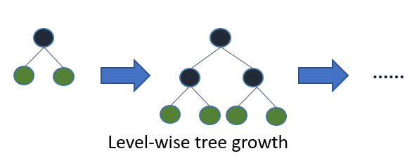
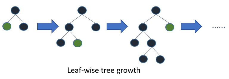
Source: LightGBM
Additionally, LightGBM uses a histogram based algorithm to discretize continuous variables into buckets in order to speed up the training process and reduce the memory requirements. XGBoost has included this in recent versions, but it is not enabled by default.
There are several other optimizations happening under the hood (listed here), but those are a few of the main differences from other implementations.
Installation
The documentation on GitHub has installation instructions for LightGBM. It can be installed from PyPI with pip install lightgbm, but requires a few things to work - check out the documentation depending on your OS.
import lightgbm as lgb

lightGBM = lgb.LGBMClassifier(nthread=-1)  # nthread=-1 uses all available cores

# Due to the scikit-learn API option, LightGBM works with our function!
train_model_get_results(lightGBM, 'LightGBM')
Training the model
Completed

 Non-tuned results:
| Accuracy | LogLoss | AUC | TrainingTime | |
|---|---|---|---|---|
| Logistic Regression | 0.530467 | 0.690443 | 0.542193 | 2.046665 |
| Random Forest | 0.576922 | 0.779316 | 0.608052 | 13.342987 |
| LightGBM | 0.585022 | 0.678384 | 0.616754 | 1.859263 |
| LightGBM AUC | 0.585022 | 0.678384 | 0.616754 | 1.765515 |
Hyperparameter Tuning
Because LightGBM is so similar to XGBoost, we can use the same tuning guidelines in principle. However, there are a few additional tuning guidelines noted in the official LightGBM Parameter Tuning Guide.
TODO: Adjust these hyperparameters
parameters = {'n_estimators': scipy.stats.randint(low=10, high=1000),  # Uniform distribution between 10 and 1000
              'learning_rate': [0.01, 0.03, 0.1, 0.3],
              'max_depth': [4, 6, 8, 10],
              'subsample': [0.5, 0.75, 1.0],
              'reg_alpha': [0, 1],  # L1 regularization
              'reg_lambda': [0, 1]  # L2 regularization
             }

hyperparameter_tune_get_results(lightGBM, parameters, 'LightGBM', num_rounds=30)
Default Parameters:

LGBMClassifier(boosting_type='gbdt', colsample_bytree=1, learning_rate=0.1,
        max_bin=255, max_depth=-1, min_child_samples=10,
        min_child_weight=5, min_split_gain=0, n_estimators=100, nthread=-1,
        num_leaves=31, objective='binary', reg_alpha=0, reg_lambda=0,
        seed=0, silent=True, subsample=1, subsample_for_bin=50000,
        subsample_freq=1)

Beginning hyperparameter tuning
Fitting 3 folds for each of 30 candidates, totalling 90 fits
[Parallel(n_jobs=-1)]: Done   5 tasks      | elapsed:  1.5min
[Parallel(n_jobs=-1)]: Done  10 tasks      | elapsed:  3.4min
[Parallel(n_jobs=-1)]: Done  17 tasks      | elapsed:  5.6min
[Parallel(n_jobs=-1)]: Done  24 tasks      | elapsed:  7.9min
[Parallel(n_jobs=-1)]: Done  33 tasks      | elapsed:  9.8min
[Parallel(n_jobs=-1)]: Done  42 tasks      | elapsed: 13.4min
[Parallel(n_jobs=-1)]: Done  53 tasks      | elapsed: 16.3min
[Parallel(n_jobs=-1)]: Done  64 tasks      | elapsed: 19.2min
[Parallel(n_jobs=-1)]: Done  77 tasks      | elapsed: 24.3min
[Parallel(n_jobs=-1)]: Done  90 out of  90 | elapsed: 27.2min finished
Completed
Best estimator:

LGBMClassifier(boosting_type='gbdt', colsample_bytree=1, learning_rate=0.03,
        max_bin=255, max_depth=6, min_child_samples=10, min_child_weight=5,
        min_split_gain=0, n_estimators=935, nthread=-1, num_leaves=31,
        objective='binary', reg_alpha=1, reg_lambda=1, seed=0, silent=True,
        subsample=0.5, subsample_for_bin=50000, subsample_freq=1)

Accuracy before tuning: 0.585022222222
Accuracy after tuning: 0.635922222222

 Tuned results:
| Accuracy | LogLoss | AUC | TrainingTime | |
|---|---|---|---|---|
| LightGBM | 0.635922 | 0.647806 | 0.676993 | 1664.384194 |

Blending
While not technically not one of the three ensemble methods, blending is a popular technique for combining the predictions of multiple models via averaging. It's easy to program, and typically has good results.
It has similar downsides as stacking - it requires more computational power, and any semblance of interpretability goes out the window.
num_models = 10

class_probabilities = []

for model in range(num_models):

    # Progress printing for every 10% of completion
    if (model+1) % (round(num_models) / 10) == 0:
        print('Training model number', model+1)

    model = lgb.LGBMClassifier(nthread=-1, n_estimators=935, learning_rate=0.03)
    model.fit(X_train, y_train)
    model_prediction = model.predict_proba(X_test)
    class_probabilities.append(model_prediction)

# Averaging the predictions for output
class_probabilities = np.asarray(class_probabilities).mean(axis=0)
predictions = np.where(class_probabilities[:, 1] > 0.5, 1, 0)

print()
print('Accuracy:', metrics.accuracy_score(y_test, predictions))
print('Log Loss:', metrics.log_loss(y_test, class_probabilities))
print('AUC:', metrics.roc_auc_score(y_test, class_probabilities[:, 1]))
Training model number 1
Training model number 2
Training model number 3
Training model number 4
Training model number 5
Training model number 6
Training model number 7
Training model number 8
Training model number 9
Training model number 10

Accuracy: 0.633433333333
Log Loss: 0.649578716595
AUC: 0.674961877427
tuned_results
| Accuracy | LogLoss | AUC | TrainingTime | |
|---|---|---|---|---|
| LightGBM | 0.635922 | 0.647806 | 0.676993 | 1664.384194 |
metrics.accuracy_score(y_test, predictions)
0.71255555555555561
tuned_results
| Accuracy | LogLoss | AUC | TrainingTime | |
|---|---|---|---|---|
| Logistic Regression | 0.688667 | 0.621084 | 0.719362 | 42.689128 |
| Random Forest | 0.713000 | 0.600420 | 0.731466 | 3247.834107 |
| Gradient Boosted Trees | 0.712556 | 0.619908 | 0.734792 | 4069.814399 |
| LightGBM | 0.708889 | 0.598696 | 0.734768 | 629.372810 |
Summary
And there we have it! We looked at different types of ensemble methods, how to tune them, and a few different frameworks for using them.