Shape analysis
Shape analysis
Quantitative Big Imaging - ETHZ: 227-0966-00L
Part 1
April 1, 2021
Anders Kaestner
Laboratory for Neutron Scattering and Imaging
Paul Scherrer Institut
Previously on QBI ...
| Image Enhancment | Segmentation | Automatic Methods |
|---|---|---|
|
Understanding value histograms Dealing with multi-valued data |
Hysteresis Method K-Means Analysis |
| Regions of Interest | Machine Learning | |
|
Contouring |
Learning Objectives
Motivation (Why and How?)
- How do we quantify where and how big our objects are?
- How can we say something about the shape?
- How can we compare objects of different sizes?
- How can we compare two images on the basis of the shape as calculated from the images?
- How can we put objects into an
- finite element simulation?
- or make pretty renderings?
Outline
- Motivation (Why and How?)
- Object Characterization
- Volume
- Center and Extents
- Anisotropy
Metrics
- Shape Tensor
- Principal Component Analysis
- Ellipsoid Representation
- Scale-free metrics
- Anisotropy, Oblateness
- Meshing
- Marching Cubes
- Isosurfaces
- Surface Area
Motivation
We have dramatically simplified our data, but there is still too much.
- We perform an experiment bone to see how big the cells are inside the tissue
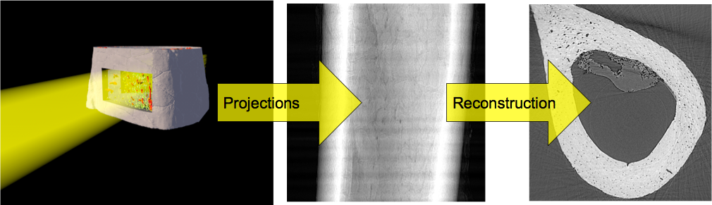
2560 x 2560 x 2160 x 32 bit 56GB / sample
- Filtering and Enhancement!
- 56GB of less noisy data
- Segmentation
2560 x 2560 x 2160 x 1 bit (1.75GB / sample)
- Still an aweful lot of data
What did we want in the first place?
Single numbers :
- volume fraction,
- cell count,
- average cell stretch,
- cell volume variability
Literature / Useful References
Jean Claude, Morphometry with R
- Online through ETHZ
John C. Russ, “The Image Processing Handbook”,(Boca Raton, CRC Press)
- Available online within domain ethz.ch (or proxy.ethz.ch / public VPN)
Principal Component Analysis
- Venables, W. N. and B. D. Ripley (2002). Modern Applied Statistics with S, Springer-Verlag
Shape Tensors
Doube, M.,et al. (2010). BoneJ: Free and extensible bone image analysis in ImageJ. Bone, 47, 1076–9. doi:10.1016/j.bone.2010.08.023
Mader, K. , et al. (2013). A quantitative framework for the 3D characterization of the osteocyte lacunar system. Bone, 57(1), 142–154. doi:10.1016/j.bone.2013.06.026
Wilhelm Burger, Mark Burge. Principles of Digital Image Processing: Core Algorithms. Springer-Verlag, London, 2009.
B. Jähne. Digital Image Processing. Springer-Verlag, Berlin-Heidelberg, 6. edition, 2005.
T. H. Reiss. Recognizing Planar Objects Using Invariant Image Features, from Lecture notes in computer science, p. 676. Springer, Berlin, 1993.
Let's load some modules for python
import numpy as np
import pandas as pd
import seaborn as sns
import matplotlib.pyplot as plt
from matplotlib.collections import PatchCollection
from matplotlib.patches     import Rectangle

from matplotlib.animation import FuncAnimation
from IPython.display      import HTML
from skimage.morphology   import label
from skimage.morphology   import erosion, disk
from skimage.measure      import regionprops
from skimage.io           import imread

from IPython.display        import Markdown, display
from sklearn.neighbors      import KNeighborsClassifier
from sklearn.decomposition  import PCA
import webcolors

from collections import defaultdict

%matplotlib inline

plt.rcParams["figure.figsize"] = (8, 8)
plt.rcParams["figure.dpi"] = 150
plt.rcParams["font.size"] = 14
plt.rcParams['font.family'] = ['sans-serif']
plt.rcParams['font.sans-serif'] = ['DejaVu Sans']
plt.style.use('default')
sns.set_style("whitegrid", {'axes.grid': False})
Once we have a clearly segmented image, it is often helpful to identify the sub-components of this image. Connected component labeling is one of the first labeling algorithms you come across. This is the easist method for identifying these subcomponents which again uses the neighborhood $\mathcal{N}$ as a criterion for connectivity. The principle of the this algorithm class is that it is it puts labels on all pixels that touch each other. This means that the algorithm searches the neighborhood of each pixel and checks if it is marked as an object. If, "yes" then the neighbor pixel will be assigned the same class a the pixels we started from. This is an iterative process until each object in the image has one unique label.
In general, the approach works well since usually when different regions are touching, they are related. It runs into issues when you have multiple regions which agglomerate together, for example a continuous pore network (1 object) or a cluster of touching cells.
- Basic component labelling
- give the same label to all pixels touching each other.
- has its drawbacks... touching item are treated as one
A cityscape image
To demonsstrate the connected components labeling we need an image. Here, we show some examples from Cityscape Data taken in Aachen (https://www.cityscapes-dataset.com/). The picture represents a street with cars in a city. The cars are also provided as a segmentation mask. This saves us the trouble of finding them in the first place.
from skimage.io import imread
import numpy as np
import matplotlib.pyplot as plt
%matplotlib inline
car_img = imread('figures/aachen_img.png')
seg_img = imread('figures/aachen_label.png')[::4, ::4] == 26
print('image dimensions', car_img.shape, seg_img.shape)
fig, (ax1, ax2) = plt.subplots(1, 2, figsize=(20, 8))
ax1.imshow(car_img)
ax1.set_title('Input Image')

ax2.imshow(seg_img, cmap='bone')
ax2.set_title('Segmented Image');
image dimensions (256, 512, 4) (256, 512)

Connected component labeling in python
from skimage.morphology import label
help(label)
Help on function label in module skimage.measure._label:

label(input, neighbors=None, background=None, return_num=False, connectivity=None)
    Label connected regions of an integer array.

    Two pixels are connected when they are neighbors and have the same value.
    In 2D, they can be neighbors either in a 1- or 2-connected sense.
    The value refers to the maximum number of orthogonal hops to consider a
    pixel/voxel a neighbor::

      1-connectivity     2-connectivity     diagonal connection close-up

           [ ]           [ ]  [ ]  [ ]             [ ]
            |               \  |  /                 |  <- hop 2
      [ ]--[x]--[ ]      [ ]--[x]--[ ]        [x]--[ ]
            |               /  |  \             hop 1
           [ ]           [ ]  [ ]  [ ]

    Parameters
    ----------
    input : ndarray of dtype int
        Image to label.
    neighbors : {4, 8}, int, optional
        Whether to use 4- or 8-"connectivity".
        In 3D, 4-"connectivity" means connected pixels have to share face,
        whereas with 8-"connectivity", they have to share only edge or vertex.
        **Deprecated, use** ``connectivity`` **instead.**
    background : int, optional
        Consider all pixels with this value as background pixels, and label
        them as 0. By default, 0-valued pixels are considered as background
        pixels.
    return_num : bool, optional
        Whether to return the number of assigned labels.
    connectivity : int, optional
        Maximum number of orthogonal hops to consider a pixel/voxel
        as a neighbor.
        Accepted values are ranging from  1 to input.ndim. If ``None``, a full
        connectivity of ``input.ndim`` is used.

    Returns
    -------
    labels : ndarray of dtype int
        Labeled array, where all connected regions are assigned the
        same integer value.
    num : int, optional
        Number of labels, which equals the maximum label index and is only
        returned if return_num is `True`.

    See Also
    --------
    regionprops

    References
    ----------
    .. [1] Christophe Fiorio and Jens Gustedt, "Two linear time Union-Find
           strategies for image processing", Theoretical Computer Science
           154 (1996), pp. 165-181.
    .. [2] Kensheng Wu, Ekow Otoo and Arie Shoshani, "Optimizing connected
           component labeling algorithms", Paper LBNL-56864, 2005,
           Lawrence Berkeley National Laboratory (University of California),
           http://repositories.cdlib.org/lbnl/LBNL-56864

    Examples
    --------
    >>> import numpy as np
    >>> x = np.eye(3).astype(int)
    >>> print(x)
    [[1 0 0]
     [0 1 0]
     [0 0 1]]
    >>> print(label(x, connectivity=1))
    [[1 0 0]
     [0 2 0]
     [0 0 3]]
    >>> print(label(x, connectivity=2))
    [[1 0 0]
     [0 1 0]
     [0 0 1]]
    >>> print(label(x, background=-1))
    [[1 2 2]
     [2 1 2]
     [2 2 1]]
    >>> x = np.array([[1, 0, 0],
    ...               [1, 1, 5],
    ...               [0, 0, 0]])
    >>> print(label(x))
    [[1 0 0]
     [1 1 2]
     [0 0 0]]
Labels in the cityscape image
When we apply the label operation on the car mask, we see the that each car is assigned a color. There are however some cars that get multiple classes. This is because they were divided into several segments due to objects like tree and trafic signs.
fig, (ax1, ax2) = plt.subplots(1, 2, figsize=(20, 8), dpi=100)
ax1.imshow(seg_img, cmap='bone')
ax1.set_title('Segmented Image')
lab_img = label(seg_img)
ax2.imshow(lab_img, cmap=plt.cm.tab10)
ax2.set_title('Labeled Image');

Area of each segment
Now, we can start making measurements in the image. A first thing that comes to mind is to compute the area of the objects. This is a very simple operation; we only have to count the number of pixels belonging to each label.
Usually, we want to know the are of all items in the images. We could do this by writing a loop that goes through all labels in the image and compute each one of them. There is however an operation that does this much easier: the histogram.
We can use a histogram with the same number of bins are there are labels in the image. This would give us the size distribution in of the objects in one single operation.
fig, (ax3) = plt.subplots(1, 1, dpi=150)
ax3.hist(lab_img.ravel())
ax3.set_title('Label Counts')
ax3.set_yscale('log')

A component labeling algorithm
We start off with all of the pixels in either foreground (1) or background (0)
seg_img = np.eye(9, dtype=int)
seg_img[4, 4] = 0
seg_img += seg_img[::-1]
sns.heatmap(seg_img, annot=True, fmt="d");

Labeling initialization
Give each point in the image a unique label
- For each point $(x,y)\in\text{Foreground}$
- Set value to $I_{x,y} = x+y*width+1$
idx_img = np.zeros_like(seg_img)
for x in range(seg_img.shape[0]):
    for y in range(seg_img.shape[1]):
        if seg_img[x, y] > 0:
            idx_img[x, y] = x+y*seg_img.shape[0]+1
sns.heatmap(idx_img, annot=True,
            fmt="d", cmap='nipy_spectral');

A brushfire labeling algorithm
In a brushfire-style algorithm
- For each point $(x,y)\in\text{Foreground}$
- For each point $(x^{\prime},y^{\prime})\in\mathcal{N}(x,y)$
- if $(x^{\prime},y^{\prime})\in\text{Foreground}$
- Set the label to $\min(I_{x,y}, I_{x^{\prime},y^{\prime}})$
- Repeat until no more labels have been changed
Implementation of the brush fire algorithm
last_img = idx_img.copy()
img_list = [last_img]
for iteration, c_ax in enumerate(m_axs.flatten(), 1):
    cur_img = last_img.copy()

    for x in range(last_img.shape[0]):
        for y in range(last_img.shape[1]):
            if last_img[x, y] > 0:
                i_xy = last_img[x, y]
                for xp in [-1, 0, 1]:
                    if (x+xp < last_img.shape[0]) and (x+xp >= 0):
                        for yp in [-1, 0, 1]:
                            if (y+yp < last_img.shape[1]) and (y+yp >= 0):
                                i_xpyp = last_img[x+xp, y+yp]
                                if i_xpyp > 0:

                                    new_val = min(i_xy, i_xpyp, cur_img[x, y])
                                    if cur_img[x, y] != new_val:
                                        print((x, y), i_xy, 'vs', (x+xp,
                                                                   y+yp), i_xpyp, '->', new_val)
                                        cur_img[x, y] = new_val

    img_list += [cur_img]
    if (cur_img == last_img).all():
        print('Done')
        break
    else:
        print('Iteration', iteration,
              'Groups', len(np.unique(cur_img[cur_img > 0].ravel())),
              'Changes', np.sum(cur_img != last_img))
        last_img = cur_img
(0, 8) 73 vs (1, 7) 65 -> 65
(1, 1) 11 vs (0, 0) 1 -> 1
(1, 7) 65 vs (2, 6) 57 -> 57
(2, 2) 21 vs (1, 1) 11 -> 11
(2, 6) 57 vs (3, 5) 49 -> 49
(3, 3) 31 vs (2, 2) 21 -> 21
(5, 3) 33 vs (6, 2) 25 -> 25
(6, 2) 25 vs (7, 1) 17 -> 17
(6, 6) 61 vs (5, 5) 51 -> 51
(7, 1) 17 vs (8, 0) 9 -> 9
(7, 7) 71 vs (6, 6) 61 -> 61
(8, 8) 81 vs (7, 7) 71 -> 71
Iteration 1 Groups 12 Changes 12
(0, 8) 65 vs (1, 7) 57 -> 57
(1, 7) 57 vs (2, 6) 49 -> 49
(2, 2) 11 vs (1, 1) 1 -> 1
(3, 3) 21 vs (2, 2) 11 -> 11
(5, 3) 25 vs (6, 2) 17 -> 17
(6, 2) 17 vs (7, 1) 9 -> 9
(7, 7) 61 vs (6, 6) 51 -> 51
(8, 8) 71 vs (7, 7) 61 -> 61
Iteration 2 Groups 8 Changes 8
(0, 8) 57 vs (1, 7) 49 -> 49
(3, 3) 11 vs (2, 2) 1 -> 1
(5, 3) 17 vs (6, 2) 9 -> 9
(8, 8) 61 vs (7, 7) 51 -> 51
Iteration 3 Groups 4 Changes 4
Done
Looking at the iterations
fig, m_axs = plt.subplots(2, 2, figsize=(15, 10)); m_axs=m_axs.ravel()
for c_ax,cur_img in zip(m_axs,img_list):
    sns.heatmap(cur_img,
                annot=True,
                fmt="d",
                cmap='nipy_spectral',
                ax=c_ax)
    c_ax.set_title('Iteration #{}'.format(iteration))

Some comments on the brushfire algorithm
The image very quickly converges and after 4 iterations the task is complete.
For larger more complicated images with thousands of components this task can take longer,
There exist much more efficient algorithms for labeling components which alleviate this issue.
Let's animate the iterations
fig, c_ax = plt.subplots(1, 1, figsize=(5, 5), dpi=100)

def update_frame(i):
    plt.cla()
    sns.heatmap(img_list[i],
                annot=True,
                fmt="d",
                cmap='nipy_spectral',
                ax=c_ax,
                cbar=False,
                vmin=img_list[0].min(),
                vmax=img_list[0].max())
    c_ax.set_title('Iteration #{}, Groups {}'.format(i+1,
                                                     len(np.unique(img_list[i][img_list[i] > 0].ravel()))))
# write animation frames
anim_code = FuncAnimation(fig, update_frame, frames=len(img_list)-1,
                          interval=1000, repeat_delay=2000).to_html5_video()
plt.close('all')
HTML(anim_code)
Bigger Images
How does the same algorithm apply to bigger images?
seg_img = (imread('figures/aachen_label.png')[::4, ::4] == 26)[110:130:2, 370:420:3]
seg_img[9, 1] = 1
_, (ax1, ax2) = plt.subplots(1, 2, figsize=(15, 7), dpi=150)
sns.heatmap(seg_img, annot=True, fmt="d", ax=ax1,
            cmap='nipy_spectral', cbar=False)
ax1.set_title('Binary image')

idx_img = seg_img * np.arange(len(seg_img.ravel())).reshape(seg_img.shape)
sns.heatmap(idx_img, annot=True, fmt="d", ax=ax2,
            cmap='nipy_spectral', cbar=False)
ax2.set_title('Initial labels');

Run the labelling on the car image
last_img = idx_img.copy()
img_list = [last_img]
for iteration in range(99):
    cur_img = last_img.copy()
    for x in range(last_img.shape[0]):
        for y in range(last_img.shape[1]):
            if last_img[x, y] > 0:
                i_xy = last_img[x, y]
                for xp in [-1, 0, 1]:
                    if (x+xp < last_img.shape[0]) and (x+xp >= 0):
                        for yp in [-1, 0, 1]:
                            if (y+yp < last_img.shape[1]) and (y+yp >= 0):
                                i_xpyp = last_img[x+xp, y+yp]
                                if i_xpyp > 0:
                                    new_val = min(i_xy, i_xpyp, cur_img[x, y])
                                    if cur_img[x, y] != new_val:
                                        cur_img[x, y] = new_val

    img_list += [cur_img] # stores the current image in the iteration list
    if (cur_img == last_img).all():
        print('Done')
        break
    else:
        print('Iteration', iteration,
              'Groups', len(np.unique(cur_img[cur_img > 0].ravel())),
              'Changes', np.sum(cur_img != last_img))
        last_img = cur_img
Iteration 0 Groups 62 Changes 79
Iteration 1 Groups 46 Changes 74
Iteration 2 Groups 32 Changes 68
Iteration 3 Groups 22 Changes 59
Iteration 4 Groups 14 Changes 46
Iteration 5 Groups 8 Changes 31
Iteration 6 Groups 5 Changes 17
Iteration 7 Groups 3 Changes 6
Iteration 8 Groups 2 Changes 1
Done
Let's animate the iterations
fig, c_ax = plt.subplots(1, 1, figsize=(5, 5), dpi=100)

def update_frame(i):
    plt.cla()
    sns.heatmap(img_list[i],
                annot=True,
                fmt="d",
                cmap='nipy_spectral',
                ax=c_ax,
                cbar=False,
                vmin=img_list[0].min(),
                vmax=img_list[0].max())
    c_ax.set_title('Iteration #{}, Groups {}'.format(i+1,
                                                     len(np.unique(img_list[i][img_list[i] > 0].ravel()))))


# write animation frames
anim_code = FuncAnimation(fig,
                          update_frame,
                          frames=len(img_list)-1,
                          interval=500,
                          repeat_delay=1000).to_html5_video()
plt.close('all')
HTML(anim_code)
Different Neighborhoods
We can expand beyond the 3x3 neighborhood to a 5x5 for example
last_img = idx_img.copy()
img_list = [last_img]
for iteration in range(99):
    cur_img = last_img.copy()
    for x in range(last_img.shape[0]):
        for y in range(last_img.shape[1]):
            if last_img[x, y] > 0:
                i_xy = last_img[x, y]
                for xp in [-2, -1, 0, 1, 2]:
                    if (x+xp < last_img.shape[0]) and (x+xp >= 0):
                        for yp in [-2, -1, 0, 1, 2]:
                            if (y+yp < last_img.shape[1]) and (y+yp >= 0):
                                i_xpyp = last_img[x+xp, y+yp]
                                if i_xpyp > 0:
                                    new_val = min(i_xy, i_xpyp, cur_img[x, y])
                                    if cur_img[x, y] != new_val:
                                        cur_img[x, y] = new_val

    img_list += [cur_img]
    if (cur_img == last_img).all():
        print('Done')
        break
    else:
        print('Iteration', iteration,
              'Groups', len(np.unique(cur_img[cur_img > 0].ravel())),
              'Changes', np.sum(cur_img != last_img))
        last_img = cur_img
Iteration 0 Groups 49 Changes 81
Iteration 1 Groups 24 Changes 71
Iteration 2 Groups 8 Changes 51
Iteration 3 Groups 2 Changes 20
Iteration 4 Groups 1 Changes 1
Done
Animate the labeling iterations
fig, c_ax = plt.subplots(1, 1, figsize=(5, 5), dpi=100)

def update_frame(i):
    plt.cla()
    sns.heatmap(img_list[i],
                annot=True,
                fmt="d",
                cmap='nipy_spectral',
                ax=c_ax,
                cbar=False,
                vmin=img_list[0].min(),
                vmax=img_list[0].max())
    c_ax.set_title('Iteration #{}, Groups {}'.format(i+1,
                                                     len(np.unique(img_list[i][img_list[i] > 0].ravel()))))

# write animation frames
anim_code = FuncAnimation(fig,
                          update_frame,
                          frames=len(img_list)-1,
                          interval=500,
                          repeat_delay=1000).to_html5_video()
plt.close('all')
HTML(anim_code)
Or a smaller kernel
By using a smaller kernel (in this case where $\sqrt{x^2+y^2}<=1$, we cause the number of iterations to fill to increase and prevent the last pixel from being grouped since it is only connected diagonally
| 0 | 1 | 0 |
| 1 | 1 | 1 |
| 0 | 1 | 0 |
last_img = idx_img.copy()
img_list = [last_img]
for iteration in range(99):
    cur_img = last_img.copy()
    for x in range(last_img.shape[0]):
        for y in range(last_img.shape[1]):
            if last_img[x, y] > 0:
                i_xy = last_img[x, y]
                for xp in [-1, 0, 1]:
                    if (x+xp < last_img.shape[0]) and (x+xp >= 0):
                        for yp in [-1, 0, 1]:
                            if np.abs(xp)+np.abs(yp) <= 1:
                                if (y+yp < last_img.shape[1]) and (y+yp >= 0):
                                    i_xpyp = last_img[x+xp, y+yp]
                                    if i_xpyp > 0:
                                        new_val = min(
                                            i_xy, i_xpyp, cur_img[x, y])
                                        if cur_img[x, y] != new_val:
                                            cur_img[x, y] = new_val

    img_list += [cur_img]
    if (cur_img == last_img).all():
        print('Done')
        break
    else:
        print('Iteration', iteration,
              'Groups', len(np.unique(cur_img[cur_img > 0].ravel())),
              'Changes', np.sum(cur_img != last_img))
        last_img = cur_img
Iteration 0 Groups 68 Changes 76
Iteration 1 Groups 54 Changes 73
Iteration 2 Groups 42 Changes 67
Iteration 3 Groups 31 Changes 62
Iteration 4 Groups 21 Changes 57
Iteration 5 Groups 13 Changes 49
Iteration 6 Groups 11 Changes 39
Iteration 7 Groups 9 Changes 34
Iteration 8 Groups 8 Changes 25
Iteration 9 Groups 7 Changes 20
Iteration 10 Groups 6 Changes 15
Iteration 11 Groups 5 Changes 10
Iteration 12 Groups 4 Changes 6
Iteration 13 Groups 3 Changes 2
Done
fig, c_ax = plt.subplots(1, 1, figsize=(6, 6), dpi=100)


def update_frame(i):
    plt.cla()
    sns.heatmap(img_list[i],
                annot=True,
                fmt="d",
                cmap='nipy_spectral',
                ax=c_ax,
                cbar=False,
                vmin=img_list[0].min(),
                vmax=img_list[0].max())
    c_ax.set_title('Iteration #{}, Groups {}'.format(i+1,
                                                     len(np.unique(img_list[i][img_list[i] > 0].ravel()))))


# write animation frames
anim_code = FuncAnimation(fig,
                          update_frame,
                          frames=len(img_list)-1,
                          interval=500,
                          repeat_delay=1000).to_html5_video()
plt.close('all')
HTML(anim_code)
Comparing different neighborhoods
| Neighborhood size | Iterations | Segments |
|---|---|---|
| 3x3 | 9 | 2 |
| 5x5 | 5 | 1 |
| cross | 14 | 3 |
Beyond component labeling - what can we measure?
Now all the voxels which are connected have the same label. We can then perform simple metrics like
- counting the number of voxels in each label to estimate volume.
- looking at the change in volume during erosion or dilation to estimate surface area
What we would like to to do
- Count the cells
- Say something about the cells
- Compare the cells in this image to another image
... But where do we start?
Object position - Center of Volume (COV): With a single object
$$ I_{id}(x,y) = \begin{cases} 1, & L(x,y) = id \\ 0, & \text{otherwise} \end{cases}$$seg_img = imread('figures/aachen_label.png') == 26
seg_img = seg_img[::4, ::4]
seg_img = seg_img[110:130:2, 370:420:3]
seg_img[9, 1] = 1
lab_img = label(seg_img)
fig, ax = plt.subplots(figsize=[8,6],dpi=100)
# Using matshow here just because it sets the ticks up nicely. imshow is faster.
ax.matshow(lab_img,cmap='viridis')
for (i, j), z in np.ndenumerate(lab_img):
ax.text(j, i, '{}'.format(z), ha='center', va='center')

Define a center
$$ \bar{x} = \frac{1}{N} \sum_{\vec{v}\in I_{id}} \vec{v}\cdot\vec{i} $$$$ \bar{y} = \frac{1}{N} \sum_{\vec{v}\in I_{id}} \vec{v}\cdot\vec{j} $$$$ \bar{z} = \frac{1}{N} \sum_{\vec{v}\in I_{id}} \vec{v}\cdot\vec{k} $$i.e. the average position of all pixels in each direction.
Center of a labeled item
x_coord, y_coord = [], []
for x in range(lab_img.shape[0]):
    for y in range(lab_img.shape[1]):
        if lab_img[x, y] == 2:
            x_coord += [x]
            y_coord += [y]
items = pd.DataFrame.from_dict({'x': x_coord, 'y': y_coord})

fig, ax = plt.subplots(1,2,figsize=[15,6],dpi=100)
# Using matshow here just because it sets the ticks up nicely. imshow is faster.
ax[1].matshow(lab_img,cmap='viridis')
ax[1].plot(np.mean(y_coord),np.mean(x_coord),'rX',
        label="x={0:0.2f}, y= {1:0.2f}".format(np.mean(x_coord), np.mean(y_coord)))
ax[1].legend()
for (i, j), z in np.ndenumerate(lab_img):
    ax[1].text(j, i, '{}'.format(z), ha='center', va='center')
pd.plotting.table(data=items, ax=ax[0], loc='center')
ax[0].set_title('Coordinates of Item 2'); ax[0].axis('off');

Center of Mass (COM): With a single object
If the gray values are kept (or other meaningful ones are used), this can be seen as a weighted center of volume or center of mass (using $I_{gy}$ to distinguish it from the labels)
Define a center
$$ \Sigma I_{gy} = \frac{1}{N} \sum_{\vec{v}\in I_{id}} I_{gy}(\vec{v}) $$$$ \bar{x} = \frac{1}{\Sigma I_{gy}} \sum_{\vec{v}\in I_{id}} (\vec{v}\cdot\vec{i}) I_{gy}(\vec{v}) $$$$ \bar{y} = \frac{1}{\Sigma I_{gy}} \sum_{\vec{v}\in I_{id}} (\vec{v}\cdot\vec{j}) I_{gy}(\vec{v}) $$$$ \bar{z} = \frac{1}{\Sigma I_{gy}} \sum_{\vec{v}\in I_{id}} (\vec{v}\cdot\vec{k}) I_{gy}(\vec{v}) $$xx, yy = np.meshgrid(np.linspace(0, 10, 50),
np.linspace(0, 10, 50))
gray_img = 100*(np.abs(xx*yy-7) + np.square(yy-4))+0.25
gray_img *= np.abs(xx-5) < 3
gray_img *= np.abs(yy-5) < 3
gray_img[gray_img > 0] += 5
seg_img = (gray_img > 0).astype(int)
_, (ax1, ax2) = plt.subplots(1, 2, figsize=(14, 6), dpi=150)
sns.heatmap(gray_img,ax=ax1, cmap='bone_r', cbar=True)
ax1.set_title('Intensity Image')
sns.heatmap(seg_img, ax=ax2, cmap='bone', cbar=False)
ax2.set_title('Segmented Image');

# Collect information
x_coord, y_coord, i_val = [], [], []
for x in range(seg_img.shape[0]):
    for y in range(seg_img.shape[1]):
        if seg_img[x, y] == 1:
            x_coord += [x]
            y_coord += [y]
            i_val   += [gray_img[x, y]]

x_coord = np.array(x_coord)
y_coord = np.array(y_coord)
i_val   = np.array(i_val)
cov_x   = np.mean(x_coord)
cov_y   = np.mean(y_coord)
com_x   = np.mean(x_coord*i_val)/i_val.mean()
com_y   = np.mean(y_coord*i_val)/i_val.mean()

_, (ax1) = plt.subplots(1, 1, figsize=(6, 6), dpi=150)

im=ax1.matshow(gray_img,cmap='bone_r'); fig.colorbar(im,ax=ax1, shrink=0.8)
ax1.set_title('Intensity Image')
ax1.plot([cov_y], [cov_x], 'ro', label='COV: $x_v=$ {0:0.2f}, $y_v=${1:0.2f}'.format(cov_x,cov_y), markersize=10)
ax1.plot([com_y], [com_x], 'bo', label='COM: $x_m=$ {0:0.2f}, $y_m=${1:0.2f}'.format(com_x,com_y), markersize=10); ax1.legend();

Further object metrics
The center tells the position of an object.
We want more! E.g. metrics like:
- Area
- Perimeter length
- Sphericity
- Orientation
... and more
regionprops gives us all this!
Regionprops manual page
from skimage.measure import regionprops
help(regionprops)
Help on function regionprops in module skimage.measure._regionprops:

regionprops(label_image, intensity_image=None, cache=True, coordinates=None)
    Measure properties of labeled image regions.

    Parameters
    ----------
    label_image : (N, M) ndarray
        Labeled input image. Labels with value 0 are ignored.

        .. versionchanged:: 0.14.1
            Previously, ``label_image`` was processed by ``numpy.squeeze`` and
            so any number of singleton dimensions was allowed. This resulted in
            inconsistent handling of images with singleton dimensions. To
            recover the old behaviour, use
            ``regionprops(np.squeeze(label_image), ...)``.
    intensity_image : (N, M) ndarray, optional
        Intensity (i.e., input) image with same size as labeled image.
        Default is None.
    cache : bool, optional
        Determine whether to cache calculated properties. The computation is
        much faster for cached properties, whereas the memory consumption
        increases.
    coordinates : DEPRECATED
        This argument is deprecated and will be removed in a future version
        of scikit-image.

        See :ref:`Coordinate conventions <numpy-images-coordinate-conventions>`
        for more details.

        .. deprecated:: 0.16.0
            Use "rc" coordinates everywhere. It may be sufficient to call
            ``numpy.transpose`` on your label image to get the same values as
            0.15 and earlier. However, for some properties, the transformation
            will be less trivial. For example, the new orientation is
            :math:`\frac{\pi}{2}` plus the old orientation.


    Returns
    -------
    properties : list of RegionProperties
        Each item describes one labeled region, and can be accessed using the
        attributes listed below.

    Notes
    -----
    The following properties can be accessed as attributes or keys:

    **area** : int
        Number of pixels of the region.
    **bbox** : tuple
        Bounding box ``(min_row, min_col, max_row, max_col)``.
        Pixels belonging to the bounding box are in the half-open interval
        ``[min_row; max_row)`` and ``[min_col; max_col)``.
    **bbox_area** : int
        Number of pixels of bounding box.
    **centroid** : array
        Centroid coordinate tuple ``(row, col)``.
    **convex_area** : int
        Number of pixels of convex hull image, which is the smallest convex
        polygon that encloses the region.
    **convex_image** : (H, J) ndarray
        Binary convex hull image which has the same size as bounding box.
    **coords** : (N, 2) ndarray
        Coordinate list ``(row, col)`` of the region.
    **eccentricity** : float
        Eccentricity of the ellipse that has the same second-moments as the
        region. The eccentricity is the ratio of the focal distance
        (distance between focal points) over the major axis length.
        The value is in the interval [0, 1).
        When it is 0, the ellipse becomes a circle.
    **equivalent_diameter** : float
        The diameter of a circle with the same area as the region.
    **euler_number** : int
        Euler characteristic of region. Computed as number of objects (= 1)
        subtracted by number of holes (8-connectivity).
    **extent** : float
        Ratio of pixels in the region to pixels in the total bounding box.
        Computed as ``area / (rows * cols)``
    **filled_area** : int
        Number of pixels of the region will all the holes filled in. Describes
        the area of the filled_image.
    **filled_image** : (H, J) ndarray
        Binary region image with filled holes which has the same size as
        bounding box.
    **image** : (H, J) ndarray
        Sliced binary region image which has the same size as bounding box.
    **inertia_tensor** : ndarray
        Inertia tensor of the region for the rotation around its mass.
    **inertia_tensor_eigvals** : tuple
        The eigenvalues of the inertia tensor in decreasing order.
    **intensity_image** : ndarray
        Image inside region bounding box.
    **label** : int
        The label in the labeled input image.
    **local_centroid** : array
        Centroid coordinate tuple ``(row, col)``, relative to region bounding
        box.
    **major_axis_length** : float
        The length of the major axis of the ellipse that has the same
        normalized second central moments as the region.
    **max_intensity** : float
        Value with the greatest intensity in the region.
    **mean_intensity** : float
        Value with the mean intensity in the region.
    **min_intensity** : float
        Value with the least intensity in the region.
    **minor_axis_length** : float
        The length of the minor axis of the ellipse that has the same
        normalized second central moments as the region.
    **moments** : (3, 3) ndarray
        Spatial moments up to 3rd order::

            m_ij = sum{ array(row, col) * row^i * col^j }

        where the sum is over the `row`, `col` coordinates of the region.
    **moments_central** : (3, 3) ndarray
        Central moments (translation invariant) up to 3rd order::

            mu_ij = sum{ array(row, col) * (row - row_c)^i * (col - col_c)^j }

        where the sum is over the `row`, `col` coordinates of the region,
        and `row_c` and `col_c` are the coordinates of the region's centroid.
    **moments_hu** : tuple
        Hu moments (translation, scale and rotation invariant).
    **moments_normalized** : (3, 3) ndarray
        Normalized moments (translation and scale invariant) up to 3rd order::

            nu_ij = mu_ij / m_00^[(i+j)/2 + 1]

        where `m_00` is the zeroth spatial moment.
    **orientation** : float
        Angle between the 0th axis (rows) and the major
        axis of the ellipse that has the same second moments as the region,
        ranging from `-pi/2` to `pi/2` counter-clockwise.
    **perimeter** : float
        Perimeter of object which approximates the contour as a line
        through the centers of border pixels using a 4-connectivity.
    **slice** : tuple of slices
        A slice to extract the object from the source image.
    **solidity** : float
        Ratio of pixels in the region to pixels of the convex hull image.
    **weighted_centroid** : array
        Centroid coordinate tuple ``(row, col)`` weighted with intensity
        image.
    **weighted_local_centroid** : array
        Centroid coordinate tuple ``(row, col)``, relative to region bounding
        box, weighted with intensity image.
    **weighted_moments** : (3, 3) ndarray
        Spatial moments of intensity image up to 3rd order::

            wm_ij = sum{ array(row, col) * row^i * col^j }

        where the sum is over the `row`, `col` coordinates of the region.
    **weighted_moments_central** : (3, 3) ndarray
        Central moments (translation invariant) of intensity image up to
        3rd order::

            wmu_ij = sum{ array(row, col) * (row - row_c)^i * (col - col_c)^j }

        where the sum is over the `row`, `col` coordinates of the region,
        and `row_c` and `col_c` are the coordinates of the region's weighted
        centroid.
    **weighted_moments_hu** : tuple
        Hu moments (translation, scale and rotation invariant) of intensity
        image.
    **weighted_moments_normalized** : (3, 3) ndarray
        Normalized moments (translation and scale invariant) of intensity
        image up to 3rd order::

            wnu_ij = wmu_ij / wm_00^[(i+j)/2 + 1]

        where ``wm_00`` is the zeroth spatial moment (intensity-weighted area).

    Each region also supports iteration, so that you can do::

      for prop in region:
          print(prop, region[prop])

    See Also
    --------
    label

    References
    ----------
    .. [1] Wilhelm Burger, Mark Burge. Principles of Digital Image Processing:
           Core Algorithms. Springer-Verlag, London, 2009.
    .. [2] B. Jähne. Digital Image Processing. Springer-Verlag,
           Berlin-Heidelberg, 6. edition, 2005.
    .. [3] T. H. Reiss. Recognizing Planar Objects Using Invariant Image
           Features, from Lecture notes in computer science, p. 676. Springer,
           Berlin, 1993.
    .. [4] https://en.wikipedia.org/wiki/Image_moment

    Examples
    --------
    >>> from skimage import data, util
    >>> from skimage.measure import label
    >>> img = util.img_as_ubyte(data.coins()) > 110
    >>> label_img = label(img, connectivity=img.ndim)
    >>> props = regionprops(label_img)
    >>> # centroid of first labeled object
    >>> props[0].centroid
    (22.72987986048314, 81.91228523446583)
    >>> # centroid of first labeled object
    >>> props[0]['centroid']
    (22.72987986048314, 81.91228523446583)
Let's try regionprops on our image
from skimage.measure import regionprops
all_regs = regionprops(seg_img, intensity_image=gray_img)
attr={}
for c_reg in all_regs:
    for k in dir(c_reg):
        if not k.startswith('_') and ('image' not in k):
            attr[k]=getattr(c_reg, k)
attr_df=pd.DataFrame.from_dict(attr, orient="index")
attr_df
| 0 | |
|---|---|
| area | 900 |
| bbox | (10, 10, 40, 40) |
| bbox_area | 900 |
| centroid | (24.5, 24.5) |
| convex_area | 900 |
| coords | [[10, 10], [10, 11], [10, 12], [10, 13], [10, ... |
| eccentricity | 0 |
| equivalent_diameter | 33.8514 |
| euler_number | 1 |
| extent | 1 |
| filled_area | 900 |
| inertia_tensor | [[74.91666666666667, -0.0], [-0.0, 74.91666666... |
| inertia_tensor_eigvals | [74.91666666666667, 74.91666666666667] |
| label | 1 |
| local_centroid | (14.5, 14.5) |
| major_axis_length | 34.6218 |
| max_intensity | 7207.62 |
| mean_intensity | 2223.91 |
| min_intensity | 41.4433 |
| minor_axis_length | 34.6218 |
| moments | [[900.0, 13050.0, 256650.0, 5676750.0], [13050... |
| moments_central | [[900.0, 0.0, 67425.0, 0.0], [0.0, 0.0, 0.0, 0... |
| moments_hu | [0.16648148148148148, 0.0, 0.0, 0.0, 0.0, 0.0,... |
| moments_normalized | [[nan, nan, 0.08324074074074074, 0.0], [nan, 0... |
| orientation | 0.785398 |
| perimeter | 116 |
| slice | (slice(10, 40, None), slice(10, 40, None)) |
| solidity | 1 |
| weighted_centroid | (29.27320794892042, 27.898230520694007) |
| weighted_local_centroid | [19.27320794892042, 17.898230520694007] |
| weighted_moments | [[2001517.0866305707, 35823614.20762183, 76860... |
| weighted_moments_central | [[2001517.0866305707, -4.3655745685100555e-09,... |
| weighted_moments_hu | [6.219233313138948e-05, 2.8996448632098516e-11... |
| weighted_moments_normalized | [[nan, nan, 3.1809307780004445e-05, -8.2096428... |
Lots of information
We can tell a lot about each object now, but...
- Too abstract
- Too specific
Ask biologists in the class if they ever asked
- "How long is a cell in the $x$ direction?"
- "how about $y$?"
Extents: With a single object
Exents or caliper lenghts are the size of the object in a given direction. Since the coordinates of our image our $x$ and $y$ the extents are calculated in these directions
Define extents as the minimum and maximum values along the projection of the shape in each direction $$ \text{Ext}_x = \left\{ \forall \vec{v}\in I_{id}: max(\vec{v}\cdot\vec{i})-min(\vec{v}\cdot\vec{i}) \right\} $$ $$ \text{Ext}_y = \left\{ \forall \vec{v}\in I_{id}: max(\vec{v}\cdot\vec{j})-min(\vec{v}\cdot\vec{j}) \right\} $$ $$ \text{Ext}_z = \left\{ \forall \vec{v}\in I_{id}: max(\vec{v}\cdot\vec{k})-min(\vec{v}\cdot\vec{k}) \right\} $$
seg_img = imread('figures/aachen_label.png') == 26
seg_img = seg_img[::4, ::4]
seg_img = seg_img[110:130:2, 378:420:3] > 0
seg_img = np.pad(seg_img, 3, mode='constant')
_, (ax1) = plt.subplots(1, 1,
                        figsize=(7, 7),
                        dpi=100)
ax1.matshow(seg_img,
            cmap='bone_r');

Finding a bounding box
x_coord, y_coord = [], []
for x in range(seg_img.shape[0]):
    for y in range(seg_img.shape[1]):
        if seg_img[x, y] == 1:
            x_coord += [x]
            y_coord += [y]
xmin = np.min(x_coord)
xmax = np.max(x_coord)
ymin = np.min(y_coord)
ymax = np.max(y_coord)
print('X -> ', 'Min:', xmin,'Max:', xmax)
print('Y -> ', 'Min:', ymin,'Max:', ymax)
X ->  Min: 4 Max: 12
Y ->  Min: 3 Max: 15
Draw the box
_, (ax1) = plt.subplots(1, 1, figsize=(7, 7), dpi=100)

ax1.matshow(seg_img, cmap='bone_r')

xw = (xmax-xmin)
yw = (ymax-ymin)

c_bbox = [Rectangle(xy=(ymin, xmin),
                    width=yw,
                    height=xw
                    )]
c_bb_patch = PatchCollection(c_bbox,
                             facecolor='none',
                             edgecolor='red',
                             linewidth=4,
                             alpha=0.5)
ax1.add_collection(c_bb_patch);

Using regionprops on real images
So how can we begin to apply the tools we have developed?
We take the original car scene from before.
car_img = np.clip(imread('figures/aachen_img.png')
                  [75:150]*2.0, 0, 255).astype(np.uint8)
lab_img = label(imread('figures/aachen_label.png')[::4, ::4] == 26)[75:150]
fig, (ax1, ax2) = plt.subplots(2, 1, figsize=(20, 8))
ax1.imshow(car_img)
ax1.set_title('Input Image');

plt.colorbar(ax2.imshow(lab_img, cmap='nipy_spectral'))
ax2.set_title('Labeled Image');

Shape Analysis
We can perform shape analysis on the image and calculate basic shape parameters for each object
all_regions = regionprops(lab_img)
fig, ax1 = plt.subplots(1, 1, figsize=(12, 6), dpi=100)
ax1.imshow(car_img)
print('Found ', len(all_regions), 'regions')
bbox_list = []
for c_reg in all_regions:
    ax1.plot(c_reg.centroid[1], c_reg.centroid[0], 'o', markersize=5)
    bbox_list += [Rectangle(xy=(c_reg.bbox[1],
                                c_reg.bbox[0]),
                            width=c_reg.bbox[3]-c_reg.bbox[1],
                            height=c_reg.bbox[2]-c_reg.bbox[0]
                            )]
c_bb_patch = PatchCollection(bbox_list,
                             facecolor='none',
                             edgecolor='red',
                             linewidth=4,
                             alpha=0.5)
ax1.add_collection(c_bb_patch);
Found 9 regions

Statistics
We can then generate a table full of these basic parameters for each object. In this case, we add color as an additional description
def ed_img(in_img):
    # shrink an image to a few pixels
    cur_img = in_img.copy()
    while cur_img.max() > 0:
        last_img = cur_img
        cur_img = erosion(cur_img, disk(1))
    return last_img

# guess color name based on rgb value
color_name_class = KNeighborsClassifier(1)
c_names = sorted(webcolors.CSS3_NAMES_TO_HEX.keys())
color_name_class.fit([tuple(webcolors.name_to_rgb(k)) for k in c_names],c_names)

reg_df = pd.DataFrame([dict(label    = c_reg.label, bbox     = c_reg.bbox,
                            area     = c_reg.area,  centroid = c_reg.centroid,
                            color    = color_name_class.predict(np.mean(car_img[ed_img(lab_img == c_reg.label)], 0)[:3].reshape((1, -1)))[0])
                       for c_reg in all_regions])

fig, m_axs = plt.subplots(np.floor(len(all_regions)/3).astype(int),3, figsize=(10,10))
for c_ax, c_reg in zip(m_axs.ravel(), all_regions):
    c_ax.imshow(car_img[c_reg.bbox[0]:c_reg.bbox[2],c_reg.bbox[1]:c_reg.bbox[3]])
    c_ax.axis('off');     c_ax.set_title('Label {} '.format(c_reg.label))

reg_df
| label | bbox | area | centroid | color | |
|---|---|---|---|---|---|
| 0 | 1 | (30, 153, 58, 202) | 1091 | (43.64527956003666, 177.82218148487627) | dimgrey |
| 1 | 2 | (33, 37, 51, 77) | 535 | (41.44299065420561, 58.7607476635514) | silver |
| 2 | 3 | (37, 370, 54, 385) | 140 | (45.871428571428574, 378.6642857142857) | darkslategray |
| 3 | 4 | (37, 387, 54, 416) | 342 | (44.86257309941521, 398.66959064327483) | darkslategray |
| 4 | 5 | (38, 431, 53, 463) | 323 | (44.526315789473685, 446.9133126934984) | darkslategray |
| 5 | 6 | (46, 469, 52, 474) | 22 | (48.63636363636363, 471.1818181818182) | dimgrey |
| 6 | 7 | (46, 475, 54, 482) | 44 | (49.09090909090909, 478.22727272727275) | dimgrey |
| 7 | 8 | (47, 492, 56, 511) | 134 | (50.992537313432834, 501.82089552238807) | powderblue |
| 8 | 9 | (48, 484, 54, 489) | 25 | (50.92, 485.76) | grey |

Object anisotropy
Anisotropy: What is it?
By definition (New Oxford American): varying in magnitude according to the direction of measurement.
It allows us to define metrics in respect to one another and thereby characterize shape.
- Is it:
- tall and skinny,
- short and fat,
- or perfectly round?
A very vague definition
It can be mathematically characterized in many different very much unequal ways (in all cases 0 represents a sphere)
$$ A_{iso1} = \frac{\text{Longest Side}}{\text{Shortest Side}} - 1 $$
$$ A_{iso2} = \frac{\text{Longest Side}-\text{Shortest Side}}{\text{Longest Side}} $$
$$ A_{iso3} = \frac{\text{Longest Side}}{\text{Average Side Length}} - 1 $$
$$ A_{iso4} = \frac{\text{Longest Side}-\text{Shortest Side}}{\text{Average Side Length}} $$
$$ \cdots \rightarrow \text{ ad nauseum} $$
from collections import defaultdict
from skimage.measure import regionprops
import seaborn as sns
import numpy as np
import matplotlib.pyplot as plt
%matplotlib inline
Let's define some of these metrics
xx, yy = np.meshgrid(np.linspace(-5, 5, 100),
                     np.linspace(-5, 5, 100))


def side_len(c_reg): return sorted(
    [c_reg.bbox[3]-c_reg.bbox[1], c_reg.bbox[2]-c_reg.bbox[0]])


aiso_funcs = [lambda x:  side_len(x)[-1]/side_len(x)[0]-1,
              lambda x: (side_len(x)[-1]-side_len(x)[0])/side_len(x)[-1],
              lambda x:  side_len(x)[-1]/np.mean(side_len(x))-1,
              lambda x: (side_len(x)[-1]-side_len(x)[0])/np.mean(side_len(x))]


def ell_func(a, b): return np.sqrt(np.square(xx/a)+np.square(yy/b)) <= 1
How does the anisotropy metrics respond?
In this demonstration, we look into how the four different anisotropy metrics respond to different radius ratios of an ellipse. The ellipse is nicely aligned with the x- and y- axes, therefore we can use the bounding box to identify the side lengths as diameters in the two directions. These side lengths will be used to compute the aniotropy with our four metrics.
Much of the code below is for the animated display.
ab_list = [(2, 2), (2, 3), (2, 4), (2, 5), (1.5, 5),
           (1, 5), (0.5, 5), (0.1, 5),  (0.05, 5)]
func_pts = defaultdict(list)

fig, m_axs = plt.subplots(2, 3, figsize=(9, 6), dpi=100)

def update_frame(i):
    plt.cla()
    a, b     = ab_list[i]
    c_img    = ell_func(a, b)
    reg_info = regionprops(c_img.astype(int))[0]
    m_axs[0, 0].imshow(c_img, cmap='gist_earth')
    m_axs[0, 0].set_title('Shape #{}'.format(i+1))
    for j, (c_func, c_ax) in enumerate(zip(aiso_funcs, m_axs.flatten()[1:]), 1):
        func_pts[j] += [c_func(reg_info)]
        c_ax.plot(func_pts[j], 'r-')
        c_ax.set_title('Anisotropy #{}'.format(j))
        c_ax.set_ylim(-.1, 3)
    m_axs.flatten()[-1].axis('off')


# write animation frames
anim_code = FuncAnimation(fig,
                          update_frame,
                          frames=len(ab_list)-1,
                          interval=500,
                          repeat_delay=2000).to_html5_video()
plt.close('all')
HTML(anim_code)
Statistical tools
Useful Statistical Tools
While many of the topics covered in
- Linear Algebra
- and Statistics courses
might not seem very applicable to real problems at first glance.
at least a few of them come in handy for dealing distributions of pixels
(they will only be briefly covered, for more detailed review look at some of the suggested material)
Principal Component Analysis - PCA
- Similar to K-Means insofar as we start with a series of points in a vector space and want to condense the information.
With PCA
- doesn't search for distinct groups,
- we find a linear combination of components which best explain the variance in the system.
To read Principal component analysis: a review and recent developments
PCA definition
- Compute the covariance or correlation matrix from a set of images
- Make an Eigen value or Singular Value Decomposition
- Use
- singular values to measure the importance of each eigen value
- eigen vectors to transform the data
PCA on spectroscopy
As an example we will use a very simple (simulated) example from spectroscopy:
cm_dm = np.linspace(1000, 4000, 300)

# helper functions to build our test data
def peak(cent, wid, h): return h/(wid*np.sqrt(2*np.pi)) * \
    np.exp(-np.square((cm_dm-cent)/wid))

def peaks(plist): return np.sum(np.stack(
    [peak(cent, wid, h) for cent, wid, h in plist], 0), 0)+np.random.uniform(0, 1, size=cm_dm.shape)

# Define material spectra
fat_curve     = [(2900, 100, 500), (1680, 200, 400)]
protein_curve = [(2900, 50, 200), (3400, 100, 600), (1680, 200, 300)]
noise_curve   = [(3000, 50, 1)]

# Plotting
fig, ax = plt.subplots(1, 4, figsize=(15, 4))
ax[2].plot(cm_dm, peaks(fat_curve));     ax[2].set_title('Fat IR Spectra')
ax[3].plot(cm_dm, peaks(protein_curve)); ax[3].set_title('Protein IR Spectra')
ax[1].plot(cm_dm, peaks(noise_curve));   ax[1].set_title('Noise IR Spectra')
ax[1].set_ylim(ax[3].get_ylim())
ax[2].set_ylim(ax[3].get_ylim())
data=pd.DataFrame({'cm^(-1)': cm_dm, 'intensity': peaks(protein_curve)}).head(8)
pd.plotting.table(data=data.round(decimals=2), ax=ax[0], loc='center'); ax[0].axis('off'); ax[0].set_title('Protein spectrum data');

Test Dataset of a number of curves
We want to sort cells or samples into groups of being
- more fat like
- or more protein like.
How can we analyze this data without specifically looking for peaks or building models?
test_data = np.stack([peaks(c_curve) for _ in range(20)
                      for c_curve in [protein_curve, fat_curve, noise_curve]], 0)
fig, (ax1, ax2) = plt.subplots(1, 2, figsize=(14, 6))

ax1.plot(test_data[:4].T, '.-')
ax1.legend(['Curve 1', 'Curve 2', 'Curve 3', 'Curve 4'])
ax1.set_title('Data curves with peaks')
ax2.scatter(test_data[:, 0], test_data[:,1], c=range(test_data.shape[0]),
            s=20, cmap='nipy_spectral')
ax2.set_title('Scatter plot of curve 1 and 2'); ax2.set_xlabel('Curve 1'); ax2.set_ylabel('Curve 2');

Fit the data with PCA
from sklearn.decomposition import PCA
pca_tool = PCA(5)
pca_tool.fit(test_data)
PCA(n_components=5)
Plot principal components
fig, (ax1, ax2) = plt.subplots(1, 2, figsize=(14, 5),dpi=100)
score_matrix = pca_tool.transform(test_data)
ax1.plot(cm_dm, pca_tool.components_[0, :], label='Component #1')
ax1.plot(cm_dm, pca_tool.components_[
         1, :], label='Component #2', alpha=pca_tool.explained_variance_ratio_[0])
ax1.plot(cm_dm, pca_tool.components_[
         2, :], label='Component #3', alpha=pca_tool.explained_variance_ratio_[1])
ax1.legend(), ax1.set_title('Components')
ax2.scatter(score_matrix[:, 0],
            score_matrix[:, 1])
ax2.set_xlabel('Component 1')
ax2.set_ylabel('Component 2');

How important is each component?
fig, ax1 = plt.subplots(1, 1, figsize=(8, 4), dpi=100)
ax1.bar(x=range(pca_tool.explained_variance_ratio_.shape[0]),
        height=100*pca_tool.explained_variance_ratio_)
ax1.set_xlabel('Components')
ax1.set_ylabel('Explained Variance (%)');

PCA in materials science
Explore crystal textures in metals.
Bragg egde imaging - the imaging technique
- Wavelength resolved neutron imaging provides spectral images
- Crystaline properties can be explored in the spectra
- Bragg edges appear when the Bragg criterion is fulfilled


data=np.load('data/tofdata.npy')
fig,ax=plt.subplots(1,3,figsize=(15,4),dpi=100)
ax[0].imshow(data.mean(axis=2), cmap='viridis'), ax[0].set_title('Average image');
ax[1].imshow(data[:,:,100], cmap='viridis'), ax[1].set_title('Single wavelength bin');
ax[2].plot(data[20:40,10:20].mean(axis=0).mean(axis=0), color='Cornflowerblue', label = 'Material');
ax[2].plot(data[0:5,40:60].mean(axis=0).mean(axis=0),   color='coral',          label = 'Air');
ax[2].plot(data[20:40,32:35].mean(axis=0).mean(axis=0), color='green',          label = 'Spacer');
ax[2].set_title('Spectra'); ax[2].set_xlabel('Wavelength bins'); ax[2].set_ylabel('Transmission'); ax[2].legend();

Prepare the data for analysis
- Rearrange the images into 1D arrays $M\times{}N\times{}T\rightarrow{}M\cdot{}N\times{}T$
fdata=data.reshape(data.shape[0]*data.shape[1],data.shape[2])
- Compute mean and standard deviation
m  = np.reshape(fdata.mean(axis=0),(1,fdata.shape[1]))
mm = np.ones((fdata.shape[0],1))*m
s  = np.reshape(fdata.std(axis=0),(1,fdata.shape[1]))
ss = np.ones((fdata.shape[0],1))*m
- Normalize data
mfdata=(fdata-mm)/ss
Run the PCA
- Initialize PCA with 5 components
pca_tool = PCA(5)
- Fit data with PCA
pca_tool.fit(mfdata)
PCA(n_components=5)
Inspect the PCA fit
score_matrix = pca_tool.transform(mfdata)

fig, ax = plt.subplots(1, 3, figsize=(15, 5),dpi=100)
ax[0].semilogy(pca_tool.explained_variance_ratio_,'o-');
ax[0].set_title('Explained variance ratio'); ax[0].set_xlabel('Principal component #')
ax[1].plot(pca_tool.components_[0, :], label='Component #1')
ax[1].plot(pca_tool.components_[1, :], label='Component #2')
ax[1].plot(pca_tool.components_[2, :], label='Component #3')
ax[1].legend(); ax[1].set_title('Components')
ax[2].scatter(score_matrix[:, 0], score_matrix[:, 1]); ax[2].set_xlabel('Component 1'); ax[2].set_ylabel('Component 2');

Improve the scatter plot
fig, ax = plt.subplots(1, 2, figsize=(15, 7),dpi=100)
ax[0].scatter(score_matrix[:, 0], score_matrix[:, 1]); ax[1].set_xlabel('Component 1'); ax[0].set_ylabel('Component 2');
ax[0].set_title(r'Marker $\alpha$=1');
ax[1].scatter(score_matrix[:, 0], score_matrix[:, 1], alpha=0.05); ax[1].set_xlabel('Component 1'); ax[1].set_ylabel('Component 2');
ax[1].set_title(r'Marker $\alpha$=0.05');

Visualize the PCAs with color coding
Inspired by PCA in materials science
# Reshape the first three principal components
cdata = score_matrix[:,:3].reshape([data.shape[0],data.shape[1],3])

# Normalize the chanels
for i in range(3) :
    cdata[:,:,i]=(cdata[:,:,i]-cdata[:,:,i].min())/(cdata[:,:,i].max()-cdata[:,:,i].min())

fig, ax = plt.subplots(1,2,figsize=(12,6), dpi=150)
ax[0].imshow(data.mean(axis=2)); ax[0].set_title('White beam image')
ax[1].imshow(cdata); ax[1].set_title('PCA enhanced image');

The PCA enhanced image does not represent a physical reality, but it can be used as a qualitative tool to guide the material analysis.
PCA and segmentation
The next step is to use the enhanced image for segmentation:
fig, ax = plt.subplots(1,2,figsize=(12,6), dpi=150)
ax[0].imshow(cdata); ax[0].set_title('PCA enhanced image');
ax[1].scatter(score_matrix[:, 0], score_matrix[:, 1], alpha=0.05); ax[1].set_xlabel('Component 1'); ax[1].set_ylabel('Component 2');
ax[1].set_title(r'Principal components');

A project task...
- Combine clustering and PCA to identify regions in the samples
Principal Component Analysis
SciKit-learn Face Analyis
Here we show a more imaging related example from the scikit-learn documentation where we do basic face analysis with scikit-learn.
from sklearn.datasets import fetch_olivetti_faces
from sklearn import decomposition
# Load faces data
try:
    dataset = fetch_olivetti_faces(
        shuffle=True, random_state=2018, data_home='.')
    faces = dataset.data
except Exception as e:
    print('Face data not available', e)
    faces = np.random.uniform(0, 1, (400, 4096))

n_samples, n_features = faces.shape
n_row, n_col = 2, 3
n_components = n_row * n_col
image_shape = (64, 64)

# global centering
faces_centered = faces - faces.mean(axis=0)

# local centering
faces_centered -= faces_centered.mean(axis=1).reshape(n_samples, -1)

print("Dataset consists of %d faces" % n_samples)
downloading Olivetti faces from https://ndownloader.figshare.com/files/5976027 to .
Dataset consists of 400 faces
def plot_gallery(title, images, n_col=n_col, n_row=n_row):
    plt.figure(figsize=(2. * n_col, 2.26 * n_row))
    plt.suptitle(title, size=16)
    for i, comp in enumerate(images):
        plt.subplot(n_row, n_col, i + 1)
        vmax = max(comp.max(), -comp.min())
        plt.imshow(comp.reshape(image_shape), cmap=plt.cm.gray,
                   interpolation='nearest',
                   vmin=-vmax, vmax=vmax)
        plt.xticks(())
        plt.yticks(())
    plt.subplots_adjust(0.01, 0.05, 0.99, 0.93, 0.04, 0.)


# #############################################################################
# List of the different estimators, whether to center and transpose the
# problem, and whether the transformer uses the clustering API.
estimators = [
    ('Eigenfaces - PCA using randomized SVD',
     decomposition.PCA(n_components=n_components, svd_solver='randomized',
                       whiten=True),
     True)]
# #############################################################################
# Plot a sample of the input data

plot_gallery("First centered Olivetti faces", faces_centered[:n_components])

# #############################################################################
# Do the estimation and plot it

for name, estimator, center in estimators:
    print("Extracting the top %d %s..." % (n_components, name))
    data = faces
    if center:
        data = faces_centered
    estimator.fit(data)

    if hasattr(estimator, 'cluster_centers_'):
        components_ = estimator.cluster_centers_
    else:
        components_ = estimator.components_
    plot_gallery(name,
                 components_[:n_components])

plt.show()
Extracting the top 6 Eigenfaces - PCA using randomized SVD...


Applied PCA: Shape Tensor
How do these statistical analyses help us?
Going back to a single cell, we have the a distribution of $x$ and $y$ values.
- are not however completely independent
- greatest variance does not normally lie in either x nor y alone.
A principal component analysis of the voxel positions, will calculate two new principal components (the components themselves are the relationships between the input variables and the scores are the final values.)
- An optimal rotation of the coordinate system
We start off by calculating the covariance matrix from the list of $x$, $y$, and $z$ points that make up our object of interest.
$$ COV(I_{id}) = \frac{1}{N} \sum_{\forall\vec{v}\in I_{id}} \begin{bmatrix} \vec{v}_x\vec{v}_x & \vec{v}_x\vec{v}_y & \vec{v}_x\vec{v}_z\\ \vec{v}_y\vec{v}_x & \vec{v}_y\vec{v}_y & \vec{v}_y\vec{v}_z\\ \vec{v}_z\vec{v}_x & \vec{v}_z\vec{v}_y & \vec{v}_z\vec{v}_z \end{bmatrix} $$We then take the eigentransform of this array to obtain the eigenvectors (principal components, $\vec{\Lambda}_{1\cdots 3}$) and eigenvalues (scores, $\lambda_{1\cdots 3}$)
$$ COV(I_{id}) \longrightarrow \underbrace{\begin{bmatrix} \vec{\Lambda}_{1x} & \vec{\Lambda}_{1y} & \vec{\Lambda}_{1z} \\ \vec{\Lambda}_{2x} & \vec{\Lambda}_{2y} & \vec{\Lambda}_{2z} \\ \vec{\Lambda}_{3x} & \vec{\Lambda}_{3y} & \vec{\Lambda}_{3z} \end{bmatrix}}_{\textrm{Eigenvectors}} * \underbrace{\begin{bmatrix} \lambda_1 & 0 & 0 \\ 0 & \lambda_2 & 0 \\ 0 & 0 & \lambda_3 \end{bmatrix}}_{\textrm{Eigenvalues}} * \underbrace{\begin{bmatrix} \vec{\Lambda}_{1x} & \vec{\Lambda}_{1y} & \vec{\Lambda}_{1z} \\ \vec{\Lambda}_{2x} & \vec{\Lambda}_{2y} & \vec{\Lambda}_{2z} \\ \vec{\Lambda}_{3x} & \vec{\Lambda}_{3y} & \vec{\Lambda}_{3z} \end{bmatrix}^{T}}_{\textrm{Eigenvectors}} $$The principal components tell us about the orientation of the object and the scores tell us about the corresponding magnitude (or length) in that direction.
seg_img = imread('figures/aachen_label.png') == 26
seg_img = seg_img[::4, ::4]
seg_img = seg_img[130:110:-2, 378:420:3] > 0
seg_img = np.pad(seg_img, 3, mode='constant')
seg_img[0, 0] = 0
_, (ax1) = plt.subplots(1, 1, figsize=(7, 7), dpi=100)
ax1.matshow(seg_img, cmap='bone_r');

Eigenvectors of the positions
_, (ax1) = plt.subplots(1, 1,
                        figsize=(7, 7),
                        dpi=100)


ax1.plot(xy_pts[:, 1]-np.mean(xy_pts[:, 1]),
         xy_pts[:, 0]-np.mean(xy_pts[:, 0]), 's', color='lightgreen', label='Points', markersize=10)
ax1.plot([0, shape_pca.explained_variance_[0]/2*shape_pca.components_[0, 1]],
         [0, shape_pca.explained_variance_[0]/2*shape_pca.components_[0, 0]], '-', color='blueviolet', linewidth=4,
         label='PCA1')
ax1.plot([0, shape_pca.explained_variance_[1]/2*shape_pca.components_[1, 1]],
         [0, shape_pca.explained_variance_[1]/2*shape_pca.components_[1, 0]], '-', color='orange', linewidth=4,
         label='PCA2')
ax1.legend();

Rotate object using eigenvectors
from sklearn.decomposition import PCA
x_coord, y_coord = np.where(seg_img > 0) # Get object coordinates
xy_pts = np.stack([x_coord, y_coord], 1) # Build a N x 2 matrix
shape_pca = PCA()
shape_pca.fit(xy_pts)
pca_xy_vals = shape_pca.transform(xy_pts)
_, (ax1) = plt.subplots(1, 1,
                        figsize=(7, 7),
                        dpi=100)
ax1.plot(pca_xy_vals[:, 0], pca_xy_vals[:, 1], 's', color='limegreen', markersize=10);

Principal Component Analysis: Take home message
- We calculate the statistical distribution individually for $x$, $y$, and $z$ and the 'correlations' between them.
- From these values we can estimate the orientation in the direction of largest variance
- We can also estimate magnitude
- These functions are implemented as
princomporpcain various languages and scale well to very large datasets.
Principal Component Analysis: Elliptical Model
While the eigenvalues and eigenvectors are in their own right useful
- Not obvious how to visually represent these tensor objects
- Ellipsoidal (Ellipse in 2D) representation alleviates this issue
Ellipsoidal Representation
- Center of Volume is calculated normally
- Eigenvectors represent the unit vectors for the semiaxes of the ellipsoid
- $\sqrt{\text{Eigenvalues}}$ is proportional to the length of the semiaxis ($\mathcal{l}=\sqrt{5\lambda_i}$), derivation similar to moment of inertia tensor for ellipsoids.
Next Time on QBI
So, while bounding box and ellipse-based models are useful for many object and cells, they do a very poor job with other samples
Why
- We assume an entity consists of connected pixels (wrong)
- We assume the objects are well modeled by an ellipse (also wrong)
What to do?
- Is it 3 connected objects which should all be analzed seperately?
- If we could divide it, we could then analyze each spart as an ellipse
- Is it one network of objects and we want to know about the constrictions?
- Is it a cell or organelle with docking sites for cell?
- Neither extents nor anisotropy are very meaningful, we need a more specific metric which can characterize