推导和实现 Softmax、KL 散度、交叉熵和 Cross Entropy Loss,最后实现一个线性分类器 $y=xW+b$做 mnist 分类。
Softmax 函数
Softmax 函数是 Logistic function 的一种泛化,所以先介绍 Logistic function。
Logistic function 形式如下:
其中 $k$ 是 Logistic function 的抖动程度,$x_0$ 是函数关于 $x=x_0$ 对称,$L$ 曲线的最大值。
当 $k=1,L=1,x_0=0$ 时,Logistic function 就是 sigmoid 函数:
sigmoid 函数已经在激活函数中介绍,满足如下性质:
$K$ 维向量经过 softmax 函数,输出归一化之后的向量可以作为 $K$ 个不同结果发生的概率,概率值和为 1,范围在 $[0,1]$。深度学习中常用于网络输出之后使用 softmax 函数输出概率。
softmax 函数公式如下:
numpy 实现 softmax 函数,输入为一个 $batch\_size\times class\_total$ 的矩阵。
import numpy as np
def softmax(input):
    exp_value = np.exp(input) #首先计算指数
    output = exp_value/np.sum(exp_value, axis=1)[:, np.newaxis] # 然后按行标准化
    return output
output = np.random.randn(2, 3)
prob = softmax(output)
output, prob
(array([[-0.33234003,  0.44697765, -1.4677743 ],
        [-1.06887423, -0.41212265, -1.07418837]]),
 array([[0.2856109 , 0.62262729, 0.09176181],
        [0.25489283, 0.49156529, 0.25354189]]))
K-L 散度和 Cross Entropy
在 如何理解K-L散度(相对熵) 已经介绍的非常详细了,看完就可以理解 K-L 散度了。下面我提出自己的理解。
K-L 散度(Kullback–Leibler divergenc,相对熵)是描述两个概率分布 $p$ 和 $q$ 差异的一种方法,$D_{KL}(p||q)$ 表示当用概率分布 $q$ 来拟合真实分布 $p$ 时,产生的信息损耗。
首先介绍 熵(Entropy),是信息论中信息的度量单位,基本公式如下:
当对数底为 $2$ 时,表示的是编码概率分布 $p$ 所需要的最少二进制位个数。
熵的大小告诉我们编码 $p$ 最少需要多少空间,而 K-L 散度则是衡量使用一个概率分布代表另一个概率分布所损失的数据量。
K-L 散度定义如下:
$p$ 为真实分布,使用 $q$ 来近似 $p$。
由公式可以看出,$D _ { K L } ( p \| q )$ 就是 $q$ 和 $p$ 对数差值的期望,所以 k-L 散度表示如下:
如果继续用 2 为底的对数计算,则 K-L 散度值表示信息损失的二进制位数。
K-L 散度不是距离,因为不符合对称性,而距离度量应该满足对称性,例如 L1、L2 距离都是对称的。
交叉熵是 $q$ 表示 $p$ 的平均编码长度。
交叉熵刚好为 熵加上 K-L 散度,所以具体公式是:
那么为什么不用 K-L 散度而是选择交叉熵呢,K-L 散度不是更直观吗?
因为 Cross Entropy 和 K-L divergence 的结果是一样的。
在机器学习中,真实分布 $p$ 是固定的,是我们给训练集打的标签,因此对 K-L 散度由交叉熵决定,求梯度的结果是一样的。更何况交叉熵计算也非常方便。
这就是交叉熵的真实含义,由交叉熵和 softmax 函数组合之后就是交叉熵损失函数。目的是最大化真是标签的概率。
接下来介绍和实现交叉熵损失函数,并训练一个线性分类器。
Cross Entropy Loss
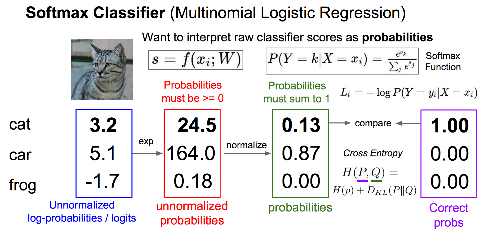
上图是交叉熵损失函数的整个流程,来源于 cs231n 的 Loss Functions and Optimization ,神经网络的输出先经过 softmax 归一化,再使用交叉熵损失函数和真实概率计算 Loss。
深度学习中使用的交叉熵损失函数形式如下,由交叉熵的公式代入 softmax 函数得来:
$y_i$ 为真实标签的 one-hot 编码,因此求和时只需要将真实标签对应的概率取对数求和即可。
因此在 Pytorch 中 torch.nn.CrossEntropyLoss 使用的是 class based 来计算 Loss,因为这样计算的速度相对于矩阵乘法更快,也节约了空间,基本公式为:
先实现交叉熵损失函数的 前向传播 过程:
N, C = 10, 3  # 随机数据,batch*class

input = np.random.randn(N, C)
from sklearn.preprocessing import OneHotEncoder
encoder = OneHotEncoder()
labels = encoder.fit_transform(np.random.randint(0, C,(N, 1))).toarray() # 生成标签并独热编码

prob = softmax(input)
# labels N*C
# prob N*C
loss = -np.sum(np.multiply(labels, np.log(prob)))/labels.shape[0] # 根据公式计算 loss,并求和
loss
1.6763745848377714
反向传播 过程需要对交叉熵损失函数计算偏导。
先对 softmax 函数求导在利用链式法则求解,对于输入 $x\in \mathcal{R}^{1\times C}$,$x=(x_0,\dots,x_i,\dots)$。
因为真实概率 $Y=(y_0,\dots,y_i,\dots)$ 为独热编码,只有一个位置为 1,所以化简 $L_i$ 为:
下标舍去,所以对 $L$ 关于 $x_i$ 求偏导为,并且 $y_i=1$:
上面只求了对于 $x_i$ 的偏导,且 $x_i$ 满足 $y_i=1$,对于 $x_j$ 且 $y_j\ne 1$,即 $y_j=0$:
$p$ 为经过 softmax 的概率,$y$ 为独热编码的矩阵,即真实概率。
所以交叉熵的梯度为 预测概率减去真实概率!
所以最后的解为:
因此最后整个反向传播过程实现就很简单了:
grad = prob - labels
grad
array([[ 0.10707167, -0.12583787,  0.01876621],
       [-0.89813245,  0.32953853,  0.56859392],
       [ 0.73705126, -0.83412744,  0.09707618],
       [ 0.1666249 , -0.90880152,  0.74217661],
       [ 0.41876515,  0.50426485, -0.92303   ],
       [-0.73118834,  0.26607816,  0.46511018],
       [-0.91878922,  0.07298688,  0.84580235],
       [ 0.68774499, -0.77065113,  0.08290614],
       [ 0.21098268, -0.75737717,  0.54639448],
       [-0.58370983,  0.51392215,  0.06978768]])
接下来就实现整个交叉熵损失函数的封装:
class CrossEntropyLossLayer():
    def __init__(self):
        pass

    def forward(self, input, labels):
        # 做一些防止误用的措施,输入数据必须是二维的,且标签和数据必须维度一致
        assert len(input.shape)==2, '输入的数据必须是一个二维矩阵'
        assert len(labels.shape)==2, '输入的标签必须是独热编码'
        assert labels.shape==input.shape, '数据和标签数量必须一致'
        self.data = input
        self.labels = labels
        self.prob = np.clip(softmax(input), 1e-9, 1.0) #在取对数时不能为 0,所以用极小数代替 0
        loss = -np.sum(np.multiply(self.labels, np.log(self.prob)))/self.labels.shape[0]
        return loss

    def backward(self):
        self.grad = (self.prob - self.labels)/self.labels.shape[0] # 根据公式计算梯度
N, C = 3, 3
data = np.random.randn(N, C)
labels = np.array([[0, 1, 0], [1, 0, 0], [0, 0, 1]], dtype=np.float32)
loss = CrossEntropyLossLayer()
l = loss.forward(data, labels)
loss.backward()
loss.grad, l
(array([[ 0.10171029, -0.21004019,  0.1083299 ],
        [-0.10804168,  0.03667105,  0.07137063],
        [ 0.14886429,  0.09000375, -0.23886804]]), 0.8824119515040371)
利用 Pytorch 的自动求导机制检验计算是否正确:
import torch
data = torch.from_numpy(data).float()
data.requires_grad = True
labels = torch.from_numpy(labels)
prob = torch.nn.functional.softmax(data, dim=1)
loss = -torch.sum(torch.mul(torch.log(prob), labels))/prob.size(0)
loss.backward()
data.grad, loss.item()
(tensor([[ 0.1017, -0.2100,  0.1083],
         [-0.1080,  0.0367,  0.0714],
         [ 0.1489,  0.0900, -0.2389]]), 0.8824119567871094)
两个结果对输入求梯度是一样的,所以我最后的答案是正确的。
只是因为精度不同有些差异,numpy 使用 64 位浮点数,而 Pytorch 使用 32 位,因为 GPU 计算单精度浮点数速度比双精度快得多。
线性分类器
实现一个线性分类器,使用交叉熵损失函数。
梯度下降更新参数,先求 $W$ 的偏导:
再根据链式法则可以求得 $L$ 关于 $W$ 的偏导:
$P$ 为 softmax 之后的预测概率,$Y$ 为独热编码的真实概率。
既然我的实现是正确的,因此读取数据:
import struct
import numpy as np
def read_mnist(filename):
    with open(filename, 'rb') as f:
        zero, data_type, dims = struct.unpack('>HBB', f.read(4))
        shape = tuple(struct.unpack('>I', f.read(4))[0] for d in range(dims))
        return np.frombuffer(f.read(), dtype=np.uint8).reshape(shape)

# 读取并归一化数据,不归一化会导致 nan
test_data = (read_mnist('../data/mnist/t10k-images.idx3-ubyte').reshape((-1, 784))-127.0)/255.0
train_data = (read_mnist('../data/mnist/train-images.idx3-ubyte').reshape((-1, 784))-127.0)/255.0
# 独热编码标签
from sklearn.preprocessing import OneHotEncoder
encoder = OneHotEncoder()
encoder.fit(np.arange(10).reshape((-1, 1)))
train_labels = encoder.transform(read_mnist('../data/mnist/train-labels.idx1-ubyte').reshape((-1, 1))).toarray()
test_labels = encoder.transform(read_mnist('../data/mnist/t10k-labels.idx1-ubyte').reshape((-1, 1))).toarray()
from nn import lr_scheduler
loss_layer = CrossEntropyLossLayer()
lr = 0.1
D, C = 784, 10
np.random.seed(1) # 固定随机生成的权重
W = np.random.randn(D, C)*0.01 # 高斯初始化,均值为 0,标准差 0.01
b = np.zeros((1, C)) # 偏置项
best_acc = -float('inf')
max_iter = 900
step_size = 400
scheduler = lr_scheduler(lr, step_size)
loss_list = []
from tqdm import tqdm_notebook
for epoch in tqdm_notebook(range(max_iter)):
    # 测试
    test_pred = np.dot(test_data, W) + b
    pred_labels = np.argmax(test_pred, axis=1)
    real_labels = np.argmax(test_labels, axis=1)
    acc = np.mean(pred_labels==real_labels)
    if acc>best_acc: best_acc=acc
    # 训练
    train_pred = np.dot(train_data, W) + b
    loss = loss_layer.forward(train_pred, train_labels)
    loss_list.append(loss)
    loss_layer.backward()
    grad = np.dot(train_data.T, loss_layer.grad)
    # 更新参数
    W -= scheduler.get_lr()*grad
    b -= scheduler.get_lr()*np.mean(loss_layer.grad, axis=0)
    scheduler.step()
best_acc
0.8992
获得了 ~90% 的准确度。绘制 Loss 曲线:
import matplotlib.pyplot as plt
plt.plot(np.arange(max_iter), loss_list)
plt.show()

使用 Pytorch 实现一个线性分类器。
import torch
train_data = torch.from_numpy(train_data).float()
train_labels = torch.from_numpy(train_labels).float()
test_data = torch.from_numpy(test_data).float()
test_labels = torch.from_numpy(test_labels).float()
# 初始化一样的权重和偏置
np.random.seed(1) # 固定随机生成的权重
linear_classifier = torch.nn.Linear(784, 10)
linear_classifier.weight.data = torch.from_numpy((np.random.randn(D, C)*0.01).transpose((1, 0))).float()
_ = linear_classifier.bias.data.fill_(0)
best_acc = -float('inf')
lr = 0.1
max_iter = 900
step_size = 400
scheduler = lr_scheduler(lr, step_size)
loss_list = []
criterion = torch.nn.CrossEntropyLoss()
for epoch in tqdm_notebook(range(max_iter)):
    with torch.no_grad():
        # 测试
        test_pred = linear_classifier(test_data)
        pred_labels = torch.argmax(test_pred, dim=1)
        real_labels = torch.argmax(test_labels, dim=1)
        acc = torch.mean((pred_labels==real_labels).float())
        if acc>best_acc: best_acc=acc
    train_pred = linear_classifier(train_data)
    real_labels = torch.argmax(train_labels, dim=1)
    loss = criterion(train_pred, real_labels)
    loss.backward()
    for p in linear_classifier.parameters():
        p.data.add_(-scheduler.get_lr(), p.grad.data)
    linear_classifier.zero_grad()
    loss_list.append(loss.item())
    scheduler.step()
best_acc
tensor(0.8992)
import matplotlib.pyplot as plt
plt.plot(np.arange(max_iter), loss_list)
plt.show()

同样的参数,获得了一样的结果,所以我的实现是完全正确的!区别在于运行速度,Pytorch 比 numpy 要快大约一倍,可能是 Pytorch 优化过矩阵预算,且单精度比双精度计算快。