Gradient Descent
Objective
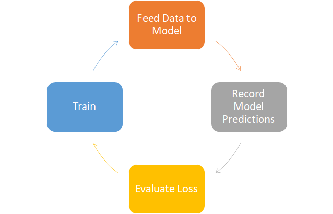
In most cases, the objective in ML and DL boil down to one thing: minimizing error.
This error is computed by feeding our model some data, recording its predictions, and feeding it to a criterion, which evaluates the performance or error of the model so that we can backpropagate/train it. We will call the operation that evaluates performance our Loss function.
Gradient Descent
There are a multitude of strategies to minimize the Loss function, all with their own unique properties; however, in DL, the objective is often approximated by some variation of Gradient Descent.
Why?
In essence, Gradient Descent is a small "step" towards the path with steepest descent (hence its name) in your model's function.
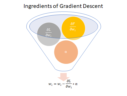
There are three main ingredients needed to take this step:
- A differentiable function/model ($\frac{\partial F}{\partial w_i}$)
- Partial of Loss function w.r.t. model parameters ($\frac{\partial L}{\partial w_i}$)
- A learning rate ($\alpha$)
Once instantiated, we formulate Gradient Descent as:
$$ w_i = w_i - \frac{\partial L}{\partial w_i} * \alpha \tag{1} $$More succinctly:
NOTE: Without a differentiable function ($\frac{\partial F}{\partial w_i}$), we would not be able to take Partial of Loss function w.r.t. model parameters ($\frac{\partial L}{\partial w_i}$)
It's a simple formulation but a powerful technique.
Now, Gradient Descent is often referred to as "stochastic" in reference to the lack of RAM storage that is needed to hold the usually large amounts of data needed to train Deep Learning models. As such, we are instead forced to create batches of (usually) randomly distributed data. When we do this, given that we are training our model on different distributions of data, our model will look like we are taking random or stochastic steps that will slowly converge to a minimum.
I mentioned that this technique "slowly" converges because gradient descent is only effective when it is constantly iterated through thousands of cycles due to the multiplication with a small $\alpha$, which forces our "step" to be tiny (I will expand more on this in the next section).
So, why does it work?
Theory
Let's revisit the definition of the derivative for a bit
$$ \frac{dy}{dx}=\lim_{h\to0}\frac{f(x+h)-f(x)}{h} \tag{2} $$From x, if we take a small forward step $h$, how much will $y$ increase/decrease by?
Traditionally, this formulation is interpreted as the velocity of the function at $x$. However, we can reformulate our expression through some algebra so lthat it can actually be interpreted as a linear approximation of $f(x+h)$ from our initial value $(x, f(x))$ to an arbitrary $x+h$.
$$ \begin{align*} & \frac{dy}{dx} = \lim_{h\to0}\frac{f(x+h)-f(x)}{h} \tag{2} \\ & \frac{dy}{dx}*\lim_{h\to0}h = f(x+h)-f(x) \\ & f(x+h) - f(x) = \frac{dy}{dx}*\lim_{h\to0}h \\ & f(x+h) = f(x) + \frac{dy}{dx}*\lim_{h\to0}h \\ & f(x+h) \approx f(x) + \frac{dy}{dx} * h \tag{3} & \end{align*} $$NOTE: the limit was taken off so as to give freedom to approximate $f(x+h)$ at any given step $h$
Does this formulation look familiar? It should! It looks *very similar* to our "step" function in gradient descent! $$ \begin{align} w_i &= w_i - \frac{\partial L}{\partial w_i} * \alpha \ (\text{Gradient Descent}) \tag{2}\\ f(x+h) &\approx f(x) + \frac{dy}{dx} * h \ (\text{Linear Approximation}) \tag{3} \end{align} $$
That is because we are applying an equal formulation to a different problem.
For Gradient Descent, instead of taking a step forward as we do with our Linear Approximation, we are actually taking a step backward (hence, the negative sign).
As a result, in Gradient Descent we are approximating the step towards steepest descend, while in our Linear Approximation, we are approximating the step towards steepest ascent.
TIP: To understand why the gradient is the direction of steepest ascent/descent, please refer to this great explanation offered by Khan Academy
Criterion
Now that we are able to attain our linear approximation of the steepest descent or ascent of our function, we must next:
- decide what Loss function we will use to compare the truth from our prediction and
- understand the relationship between our Loss function and alpha $\alpha$
Let us treat our problem as one of regression and use the Squared Error (SE) to compute the Loss of our prediction based on the truth: $$ \begin{align} \text{Squared Error} &= (f(x) + \frac{dy}{dx}h-f(x+h))^2 \ (\text{Steepest Ascent}) \tag{4} \\ \text{Squared Error} &= (f(x) - \frac{dy}{dx}h-f(x+h))^2 \ (\text{Steepest Descent}) \tag{5} \end{align} $$
The definition of the derivative we saw earlier assumes the following:
$h\to 0$, $\text{Error}\to0$
Conversely, if we are approximating a non-linear function, below is generally true:
$h\to\infty$, $Error\to\infty$
Let us display this concept with a simple example of approximating any step of $f(x+h)$ from $x=4$ by modeling $f(x)=x^2$
fig1.show()
NOTE: All visualizations can be found at the end of this notebook
The further of a step $h$ we make from $x=4$, the higher is our Squared Error! Conversely, however, when we take a small step, our squared error is minimized.
Now, keep in mind that from the perspective of Gradient Descent, we (usually) do *not calculate the Error of our linear approximation* as shown above.
Personally, this is due to the following:
- Our objective is to minimize the error w.r.t. our model's predictions from the truth, not calculate the error associated with our Gradient Descent "step"
- Calculating the
Hence, despite just taking a small step "as is" in gradient descent, we want to minimize our error so as to accurately converge to our local minima.
The Trade-Off
Given that a small step $h$ minimizes our modeling error, it follows to place a small learning $\alpha$ while performing Gradient Descent. However, a very small $\alpha$ may take hundreds or thousands of iterations more to reach a local minima. This is very problematic when our model is a "deep" network that takes much computation time to compute (as most up-to-date models are)
Hence, when setting $\alpha$ for our learning rate, we must have a trade-off between our
- Tolerance of error and
- The time it takes to reach anything close to our local minima
Let's view below animations to get a better understanding of these concepts
fig2.show()
First, notice that as the graphs progress, the learning rate of .1 converges significantly faster than both .01 and .001, despite having a higher level of tolerance for error.
Second, as learning rates begin to reach the global minima, convergence begins to plateau as the rate $dy/dx$ begins to decrease (thereby leading to smaller changes)
Third, while it may seem intuitive to place a high learning rate to our "well-behaved" quadratic function, in practice, the higher level of tolerance may lead us to "overshoot" our local minima.

Hence, when inserting $\alpha$, we must find that "golden mean" where our progression is not too fast nor too slow. There is no methodological way to find this other than pure trial and error. However, careful thought should go on in placing learning rates as computer power may restrict us to efficiently experiment between two or three learning rates.
Experiment
Now that we have defined Gradient Descent, we will showcase its performance on booth's function, which is categorized as a Plate function.
We will:
- Create a class object that holds the forward and backward pass of the function,
- Perform gradient descent at $\alpha=.01$ for 150 epochs and
- Graph our results
NOTE: The code that performed the above steps is found at the end of this notebook.
Now, let us visualize our results
fig.show()
From the above visualizations, we can tell that Gradient Descent worked well! At 150 epochs, we reached the local minima of our plate function.
Newton's Method
Again, Gradient Descent is a very simple function that relies on heavy iterations to reach a local minima. However, are there other methods?
Yes, Newton's method is one of them.
Newton's method uses the equivalent formulation of Gradient Descent, however, it applies it differently.
In a nutshell, Newton's method is the same derivation of Gradient Descent, however, this time applied to the derivative of the function such as shown below:
$$ \nabla f(x+h) \approx \nabla f(x) + \nabla^2f(x)h $$Now, what makes Newton's method truly unique is that it approximates the step $h$ needed to *reach the root of our gradient function* such as shown below:
$$ 0 = \nabla f(x+h) \approx \nabla f(x) + \nabla^2f(x)h $$Then, solving for step $h$ we get:
$$ h=-(\nabla^2f(x))^{-1}\nabla f(x) $$Let us shown an animation that represents a "step" in Newton's method
fig3.show()
Already, just one-step of Newton's Method greatly approximates the global minima.
From this perspective, Newton's method is no doubt superior than gradient descent. However, how come it is not widely applied in DL?
Newton's method forces us to compute the Hessian matrix, which is very expensive. The cost of computation coupled with some divergence problems has refrained most users from this approach.
Although there have been remedies of approximating the Hessian matrix for a boost in calculation speed, it remains to be a difficult to control optimization algorithm.
Conclusion
Optimization algorithms represent the "training" phase of DL. It is crucial to understand such an important concept, especially when it becomes a "very easy" function to implement on frameworks like PyTorch or TensorFlow.
An understanding will expand the realm of new possible training algorithms that are waiting to be found and will ensure the user to make "well-informed" decisions of our learning rate parameter.
That's it for this tutorial! Below this cells is a "Graph" section where one can find all the codes that were used for graphing.
Where to Next?
Activation Functions Tutorial: https://nbviewer.jupyter.org/github/Erick7451/DL-with-PyTorch/blob/master/Jupyter_Notebooks/ReLU.ipynb
Graphs
import numpy as np
from plotly.subplots import make_subplots
import plotly.graph_objects as go
import torch
"Linear Approximation of f(x+h) from x = 4" Graph
x = np.arange(-10,10,.1)
y = x**2
fig1 = go.Figure(
data =
[
go.Scatter(x=x,y=y, name = '$f(x)=x^2$')
],
layout = dict(
xaxis = dict(
tickmode = 'linear',
tick0 = -10,
dtick = 2,
range = [-10,10]
),
yaxis = dict(
range = [-60,60])
)
)
# add tangent line of f(x) = x^2 at x = 4
tangent = 8*x -16
fig1.add_scatter(x = x,
y = tangent,
name = 'tangent at x=4',
line_color = 'crimson')
# add two traces per slider level
for step in x:
y = step**2
yhat = 8*step -16
SE = (yhat - y)**2
# add a marker on the current x level
fig1.add_scatter(
mode = 'markers',
x = [step],
y = [yhat],
line_color = 'red',
visible = False, # do not make it visible
showlegend = False,
name = 'x = {step:.2f}'.format(step = step)) # do not show label
# add black horizontal line calculating the Squared Error
fig1.add_scatter(
x = [step,step],
y = [yhat,y],
mode = 'lines',
visible = False,
name = 'SE: {SE:.2f}'.format(SE = SE),
showlegend = False,
line = dict(
color = 'black',
width = 2,
dash = 'dot'))
# To start out, make 1st, 2nd, and 10th trace visible
fig1.data[0].visible = True
fig1.data[1].visible = True
#fig.data[2].visible = True
fig1.data[202].visible = True
fig1.data[202].showlegend = True
fig1.data[203].visible = True
fig1.data[203].showlegend = True
# with restyle method, configure each step to have all other traces set to False
steps = []
# for every step, we have a unique set of traces that we want to show
for i in range(0,len(x)*2,2):
# given that we have 2 unique traces for each step,
# we will step by 2 to change the attributes of both traces in 1 step
# the 'restyle' method controls all of the trace's attribute
# 'visible.' Below, we change all 'visible' attributes to False (except for 1st 2)
step = dict(# change attribute of traces
method = 'update',
# make sure to pass as many list elements as you have
# number of total traces. The idx of each list value
# represents the attr. element of the idx trace
args = [{'visible': [True,True]+[False] * (len(x)*2),
'showlegend': [True,True]+[False]*(len(x)*2)}]
#label = ''
)
# if all args are False,
# make 1st two traces visible
# step['args'][1][0] = True
# step['args'][1][1] = True
# make step i visible
step['args'][0]['visible'][i] = True # make marker visible
step['args'][0]['visible'][i+1] = True # make SE visible
step['args'][0]['showlegend'][i] = True
step['args'][0]['showlegend'][i+1] = True # turns SE OFF
steps.append(step)
# NOTE: step values do not need to match the number of traces
# since we have two fixed traces that we always want to show,
# we do not create steps for them
# create slider
## Out of all the steps, begin slider at step 90
sliders = [dict(active = 90,
steps = steps,
currentvalue = {'prefix': r'h: '}
)]
fig1.layout.update(sliders = sliders,
updatemenus = [go.layout.Updatemenu(showactive = True)],
title = "Linear Approximation of f(x+h) from x = 4")
# label slider steps
steps_x = np.round(x-4.1,2)
for i,step_x in enumerate(steps_x):
fig1.layout.sliders[0].steps[i].label = step_x
#fig1.show()
"Gradient Descent at Distinct Learning Rates" Graph
# model progression of distinct learning rates on f(x) = x^2
def x_squared_grad(x,alpha):
return x - (2*x*alpha)
steps1 = [4]
steps2 = [4]
steps3 = [4]
x1 = x2 = x3 = 4.0 # starting values
for epoch in range(100):
# lr with .01
x1 = x_squared_grad(x1, .1)
steps1.append(x1)
# lr with .01
x2 = x_squared_grad(x2, .01)
steps2.append(x2)
# lr with .01
x3 = x_squared_grad(x3, .001)
steps3.append(x3)
# convert x's to array
x1 = np.array(steps1)
y1 = x1**2
x2 = np.array(steps2)
y2 = x2**2
x3 = np.array(steps3)
y3 = x3**2
# frames for animation on three subplots
frames = [dict(
data=[
go.Scatter(name = 'step: '+str(i),x= [x1[i]] ,y= [y1[i]],mode='markers',marker=dict(color='red',size=8),showlegend = True),
go.Scatter(x= [x2[i]] ,y= [y2[i]],mode='markers',marker=dict(color='red',size=8),showlegend = False),
go.Scatter(x= [x3[i]] ,y= [y3[i]],mode='markers',marker=dict(color='red',size=8),showlegend = False)
],
traces = [0,1,2] # we want to update trace 0,1,2 with the above while keeping all other graphs fixed
) for i in range(len(x1))]
x = np.arange(-10,10,.1)
y = x**2
# print grid gives a unique name to each axis of the subplot
fig2 = make_subplots(print_grid = True,
shared_xaxes = True,
shared_yaxes = True,
rows=1, cols=3,
subplot_titles = ('Learning Rate: .1', 'Learning Rate: .01','Learning Rate: .001'))
## Below are fixed graphs that we want in each of the three subplots
## We will turn off the legend on each fixed graph. Once all graphs are added to fig2, we will turn one legend
## on for each fixed graph so as to attain one unique legend per fixed graph, not three (one for each subplot)
# Starting marker at (4, 16)
tangent_plot = go.Scatter(x = [4],
y = [16],
name = 'Starting Point at x=4',
marker = dict(color = 'black'),
mode = 'markers',
showlegend = False)
# f(x) = x^2 plot
x_squared_plot = go.Scatter(x=x,y=y, name = '$f(x)=x^2$',mode='lines',line=dict(width=2,color='blue'),showlegend=False)
# global minima annotation
global_minima = go.Scatter(showlegend = False,x=[-4,4],y = [0,0],mode='lines',line=dict(width=1,color='black'))
# place above three graphs in EACH subplot
fixed_traces = [tangent_plot,tangent_plot,tangent_plot, x_squared_plot,x_squared_plot,x_squared_plot,global_minima,global_minima,global_minima]
# add all fixed graphs to the corresponding subplots
fig2.add_traces(data = fixed_traces, rows = [1,1,1,1,1,1,1,1,1],cols=[1,2,3,1,2,3,1,2,3])
# for every fixed graph, turn off legend for first 2 fixed plots so that legend won't show up three times
fig2.data[0].showlegend = True
fig2.data[3].showlegend = True
#fig2.data[6].showlegend = True
layout = dict(
xaxis = dict(
tickmode = 'linear',
autorange = False,
tick0 = -10,
dtick = 2,
zeroline = False,
range = [-10,10]
),
yaxis = dict(
autorange = False,
zeroline = False,
range = [-60,60]
),
# instantiate "Play" button and indicate that we will be making an animation
updatemenus=[dict(
type = 'buttons',
buttons=[
dict(
label = 'Play',
method = 'animate',
args = [None]
)
]
)
]
)
fig2.update_layout(layout,
title_text='Gradient Descent at Distinct Learning Rates')
fig2.update(frames = frames)
fig2.update_xaxes(range=[-10,10], dtick = 2)
# global minima annotations
global_minima_annotations = (
dict(
x=0,
xref='x',
yref='y',
y=0,
text = 'Global Minima',
ax=0,
ay=-40,
font = dict(size = 9),
showarrow = True),
dict(x=0,
xref='x2',
yref='y2',
text = 'Global Minima',
font = dict(size = 9),
ax=0,
ay=-40,
showarrow = True),
dict(x=0,
xref='x3',
yref='y3',
font = dict(size = 9),
text = 'Global Minima',
ax=0,
ay=-40,
showarrow = True)
)
# extend global minima annotations to inherent annotations that make up subplot titles
# if we do not extend, titles will dissappear and our minima annotations will remain
fig2.layout.annotations = fig2.layout.annotations + global_minima_annotations
# redraw maintains or replaces legend of frames
speed = [None, dict(frame = dict(duration = 300, redraw=True), # duration of animation
transition = dict(duration = 0),#duration between old => new frame
easing = 'linear', # how to ease from old=>new frame
fromcurrent = True,
mode = 'immediate')]
fig2.layout.updatemenus[0].buttons[0].args = speed
#fig2.show()
This is the format of your plot grid: [ (1,1) x,y ] [ (1,2) x2,y2 ] [ (1,3) x3,y3 ]
Gradient Descent Booth Function
import torch
class booth():
def __init__(self):
''
# booth function
def booth(self,x,y):
return (x + 2*y - 7)**2 + (2*x + y - 5)**2
# \partial booth / \partial parameters
def partial_booth(self):
self.x = x
self.y = y
partial_x = 2*(x + 2 * y - 7) + 4*(2*x + y - 5)
partial_y = 4*(x + 2 * y - 7) + 2*(2*x + y -5)
return partial_x, partial_y
# forward pass
def forward(self,x,y):
self.x = x
self.y = y
return self.booth(x,y)
# backward pass
def backward(self):
partial_x, partial_y = self.partial_booth()
# insert calculated gradients on original tensor inputs
self.x.grad = partial_x
self.y.grad = partial_y
x = torch.FloatTensor([1])
y = torch.FloatTensor([1])
print(f"input x: {x}")
print('-'*20)
print(f"input y: {y}")
print('-'*20)
m = booth()
print(f"Foward pass: {m.forward(x,y)}")
print('-'*25)
m.backward()
print(f"Partial x Backward pass: {x.grad}")
print('-'*40)
print(f"Partial y Backward pass: {y.grad}")
input x: tensor([1.]) -------------------- input y: tensor([1.]) -------------------- Foward pass: tensor([20.]) ------------------------- Partial x Backward pass: tensor([-16.]) ---------------------------------------- Partial y Backward pass: tensor([-20.])
# implement SGD
def SGD(params: 'array-like structure', lr: float = .01):
# iterate through every parameter in our model
for p in params:
# if gradient is not required for parameter, continue
if p.grad is None:
continue
# extract the gradient of our function
p_grad = p.grad
# perform "step" inplace: p + (p_grad * -lr)
p.add_(p_grad, alpha = -lr)
# zero-out gradient inplace to calculate next forward/backward pass
p.grad.zero_()
# perform "step"
SGD([x,y], lr = .01)
print(f"Updated x: {x}")
print('-'*20)
print(f"Updated y: {y}")
Updated x: tensor([1.1600]) -------------------- Updated y: tensor([1.2000])
# now, let's perform gradient descent
#torch.manual_seed(0)
#x,y = torch.randn((2))
x = torch.FloatTensor([-5])
y = torch.FloatTensor([-5])
# record coordinates
coords = {'x': [],
'y': [],
'loss':[]}
for i in range(150):
loss = m.forward(x,y)
coords['x'].append(x.item())
coords['y'].append(y.item())
coords['loss'].append(loss.item())
# print every 5 steps
if i % 5 == 0:
print(f"Loss {i}: {loss}")
print('-'*30)
m.backward()
SGD([x,y], lr = .01)
Loss 0: tensor([884.]) ------------------------------ Loss 5: tensor([122.8633]) ------------------------------ Loss 10: tensor([17.9979]) ------------------------------ Loss 15: tensor([3.3812]) ------------------------------ Loss 20: tensor([1.2062]) ------------------------------ Loss 25: tensor([0.7716]) ------------------------------ Loss 30: tensor([0.6011]) ------------------------------ Loss 35: tensor([0.4871]) ------------------------------ Loss 40: tensor([0.3974]) ------------------------------ Loss 45: tensor([0.3246]) ------------------------------ Loss 50: tensor([0.2652]) ------------------------------ Loss 55: tensor([0.2167]) ------------------------------ Loss 60: tensor([0.1771]) ------------------------------ Loss 65: tensor([0.1447]) ------------------------------ Loss 70: tensor([0.1182]) ------------------------------ Loss 75: tensor([0.0966]) ------------------------------ Loss 80: tensor([0.0789]) ------------------------------ Loss 85: tensor([0.0645]) ------------------------------ Loss 90: tensor([0.0527]) ------------------------------ Loss 95: tensor([0.0431]) ------------------------------ Loss 100: tensor([0.0352]) ------------------------------ Loss 105: tensor([0.0287]) ------------------------------ Loss 110: tensor([0.0235]) ------------------------------ Loss 115: tensor([0.0192]) ------------------------------ Loss 120: tensor([0.0157]) ------------------------------ Loss 125: tensor([0.0128]) ------------------------------ Loss 130: tensor([0.0105]) ------------------------------ Loss 135: tensor([0.0086]) ------------------------------ Loss 140: tensor([0.0070]) ------------------------------ Loss 145: tensor([0.0057]) ------------------------------
import numpy as np
x_grid = np.arange(-5,5,.5)
y_grid = np.arange(-5,5,.5)
xx, yy = np.meshgrid(x_grid,y_grid, sparse = False)
Z = m.forward(xx, yy)
from plotly.subplots import make_subplots
import plotly.graph_objects as go
fig = make_subplots(
rows = 1, cols = 2,
shared_yaxes = True,
specs=[[{'type':'surface'},{'type':'contour'}]],
subplot_titles = ('Surface Gradient Descent','Contour Gradient Descent'))
fig.add_trace(go.Contour(z = Z,x = x_grid, y = y_grid ),row=1,col=2)
fig.add_scatter(x = coords['x'],
y = coords['y'],
mode = 'lines+text',
text = list(range(1,10)),
textposition='top left',
textfont = dict(color ='goldenrod' ),
hovertext = ['Epoch '+str(i) for i in range(1,10)],row=1,col=2)
fig.add_scatter(x = [coords['x'][-1]],
y = [coords['y'][-1]],
mode = 'lines+text',
text = ['150'],
textposition='top left',
textfont = dict(color ='goldenrod' ),
hovertext = ['Epoch 150'])
fig.add_trace(go.Surface(
contours =
{
'x': {'show': True, 'start': -5,'end':5,'size':1,'color':'black'},
'z': {'show': True, 'start': -5,'end':5,'size':1,'color':'black'}
},
x = xx,
y = yy,
z = Z,
showscale = False
),row=1,col=1)
# superimpose 3d scatterplot
fig.add_trace(go.Scatter3d(x=coords['x'],
y = coords['y'],
z = coords['loss'],
mode = 'lines+markers+text',
line_color = 'red',
marker = dict(
size = 2)
),row=1,col=1)
# add labels to the 1st 10 scatterplot coordinates
labels = [dict(font = dict(color='black'),xanchor = 'center',yanchor = 'bottom',showarrow=False,text=i+1,x=coords['x'][i],y=coords['y'][i],z=coords['loss'][i]) for i in range(9)]
# add label to last scatterplot coordinate
labels.append(dict(xanchor = 'center',yanchor = 'bottom',showarrow=False,text=150,x=coords['x'][-1],y=coords['y'][-1],z=coords['loss'][-1]))
# annotate coordinates, change z-axis name, and position camera to desired pov
fig.update_layout(
scene = dict(
annotations = labels,
zaxis_title = 'Loss',
xaxis = dict(backgroundcolor = 'rgb(200,200,230)'),
yaxis = dict(backgroundcolor = 'rgb(200,200,230)'),
zaxis = dict(backgroundcolor = 'rgb(200,200,230)')
),
scene_camera = dict(
eye = dict(x=-.4,y=1.5,z=.5))
)
fig.update_layout(showlegend = False,
yaxis = dict(range = [-5,4.5]),
xaxis = dict(range = [-5,4.5]))
Individual Contour Map
import plotly.graph_objects as go
# instantiate contour map
fig = go.Figure(data =
go.Contour(z = Z,
x = x_grid, y = y_grid )
)
# add scatterplot
fig.add_scatter(x = coords['x'],
y = coords['y'],
mode = 'lines+text',
text = list(range(1,11)),
textposition='top left',
textfont = dict(color ='goldenrod' ),
hovertext = ['Epoch '+str(i) for i in range(1,11)])
# add last step label
fig.add_scatter(x = [coords['x'][-1]],
y = [coords['y'][-1]],
mode = 'lines+text',
text = ['150'],
textposition='top left',
textfont = dict(color ='goldenrod' ),
hovertext = ['Epoch 150'])
fig.update_layout(
showlegend = False,
title_text = "Contour Map of Gradient Descent",
yaxis = dict(range = [-5,4.5]),
xaxis = dict(range = [-5,4.5]))
fig.show()
"Newton's Method" Graph
x = np.arange(-10,10,.1)
y = x**2
# Instantiate f(x) = x^2 graph
fig3 = go.Figure(
data =
[
go.Scatter(x=x,y=y, name = '$f(x)=x^2$')
],
layout = dict(
xaxis = dict(
tickmode = 'linear',
tick0 = -10,
dtick = 2,
range = [-10,10]
),
yaxis = dict(
range = [-60,60])
)
)
# add tangent line of f(x) at x = 4
tangent = 8*x -16
fig3.add_scatter(x = x,
y = tangent,
name = 'tangent at x=4',
line = dict(
color = 'crimson')
)
# add vertical line from root of linear approximation to target
fig3.add_scatter(x = [2,2],
y = [0,4],
name = 'New Displacement',
line = dict(
color = 'black')
)
# add vertical line from root of linear approximation to target
fig3.add_scatter(x = [4,2],
y = [16,0],
name = 'Newton\'s step at x = 4',
line = dict(
color = 'brown',
dash = 'dot')
)
annotations = (dict(
x=0,
xref='x',
yref='y',
y=0,
text = 'Global Minima',
ax=0,
ay=-40,
font = dict(size = 12),
showarrow = True),)
fig3.layout.annotations = annotations
fig3.layout.title = "One-Step Newton\'s Method"
Newton's Method Booth Function
import torch
class booth():
def __init__(self):
''
# booth function
def booth(self,x,y):
return (x + 2*y - 7)**2 + (2*x + y - 5)**2
# \partial booth / \partial parameters
def partial_booth(self):
self.x = x
self.y = y
partial_x = 2*(x + 2 * y - 7) + 4*(2*x + y - 5)
partial_y = 4*(x + 2 * y - 7) + 2*(2*x + y -5)
return partial_x, partial_y
def hessian(self):
self.x = x
self.y = y
hessian_x =
# forward pass
def forward(self,x,y):
self.x = x
self.y = y
return self.booth(x,y)
# backward pass
def backward(self):
partial_x, partial_y = self.partial_booth()
# insert calculated gradients on original tensor inputs
self.x.grad = partial_x
self.y.grad = partial_y
x = torch.FloatTensor([1])
y = torch.FloatTensor([1])
print(f"input x: {x}")
print('-'*20)
print(f"input y: {y}")
print('-'*20)
m = booth()
print(f"Foward pass: {m.forward(x,y)}")
print('-'*25)
m.backward()
print(f"Partial x Backward pass: {x.grad}")
print('-'*40)
print(f"Partial y Backward pass: {y.grad}")
input x: tensor([1.]) -------------------- input y: tensor([1.]) -------------------- Foward pass: tensor([20.]) ------------------------- Partial x Backward pass: tensor([-16.]) ---------------------------------------- Partial y Backward pass: tensor([-20.])
# implement SGD
def SGD(params, lr = .01):
for p in params:
if p.grad is None:
continue
p_grad = p.grad
# p + (p_grad * -lr) inplace
p.add_(p_grad, alpha = -lr)
# zero-out gradient inplace to calculate next forward/backward pass
p.grad.zero_()
# perform "step"
SGD([x,y], lr = .01)
print(f"Updated x: {x}")
print('-'*20)
print(f"Updated y: {y}")
Updated x: tensor([1.1600]) -------------------- Updated y: tensor([1.2000])
# now, let's perform gradient descent
#torch.manual_seed(0)
#x,y = torch.randn((2))
x = torch.FloatTensor([-5])
y = torch.FloatTensor([-5])
# record coordinates
coords = {'x': [],
'y': [],
'loss':[]}
for i in range(150):
loss = m.forward(x,y)
coords['x'].append(x.item())
coords['y'].append(y.item())
coords['loss'].append(loss.item())
# print every 5 steps
if i % 5 == 0:
print(f"Loss {i}: {loss}")
print('-'*30)
m.backward()
SGD([x,y], lr = .01)
Loss 0: tensor([884.]) ------------------------------ Loss 5: tensor([122.8633]) ------------------------------ Loss 10: tensor([17.9979]) ------------------------------ Loss 15: tensor([3.3812]) ------------------------------ Loss 20: tensor([1.2062]) ------------------------------ Loss 25: tensor([0.7716]) ------------------------------ Loss 30: tensor([0.6011]) ------------------------------ Loss 35: tensor([0.4871]) ------------------------------ Loss 40: tensor([0.3974]) ------------------------------ Loss 45: tensor([0.3246]) ------------------------------ Loss 50: tensor([0.2652]) ------------------------------ Loss 55: tensor([0.2167]) ------------------------------ Loss 60: tensor([0.1771]) ------------------------------ Loss 65: tensor([0.1447]) ------------------------------ Loss 70: tensor([0.1182]) ------------------------------ Loss 75: tensor([0.0966]) ------------------------------ Loss 80: tensor([0.0789]) ------------------------------ Loss 85: tensor([0.0645]) ------------------------------ Loss 90: tensor([0.0527]) ------------------------------ Loss 95: tensor([0.0431]) ------------------------------ Loss 100: tensor([0.0352]) ------------------------------ Loss 105: tensor([0.0287]) ------------------------------ Loss 110: tensor([0.0235]) ------------------------------ Loss 115: tensor([0.0192]) ------------------------------ Loss 120: tensor([0.0157]) ------------------------------ Loss 125: tensor([0.0128]) ------------------------------ Loss 130: tensor([0.0105]) ------------------------------ Loss 135: tensor([0.0086]) ------------------------------ Loss 140: tensor([0.0070]) ------------------------------ Loss 145: tensor([0.0057]) ------------------------------
import numpy as np
x_grid = np.arange(-5,5,.5)
y_grid = np.arange(-5,5,.5)
xx, yy = np.meshgrid(x_grid,y_grid, sparse = False)
Z = m.forward(xx, yy)
from plotly.subplots import make_subplots
import plotly.graph_objects as go
fig = make_subplots(
rows = 1, cols = 2,
shared_yaxes = True,
specs=[[{'type':'surface'},{'type':'contour'}]],
subplot_titles = ('Surface Gradient Descent','Contour Gradient Descent'))
fig.add_trace(go.Contour(z = Z,x = x_grid, y = y_grid ),row=1,col=2)
fig.add_scatter(x = coords['x'],
y = coords['y'],
mode = 'lines+text',
text = list(range(1,10)),
textposition='top left',
textfont = dict(color ='goldenrod' ),
hovertext = ['Epoch '+str(i) for i in range(1,10)],row=1,col=2)
fig.add_scatter(x = [coords['x'][-1]],
y = [coords['y'][-1]],
mode = 'lines+text',
text = ['150'],
textposition='top left',
textfont = dict(color ='goldenrod' ),
hovertext = ['Epoch 150'])
fig.add_trace(go.Surface(
contours =
{
'x': {'show': True, 'start': -5,'end':5,'size':1,'color':'black'},
'z': {'show': True, 'start': -5,'end':5,'size':1,'color':'black'}
},
x = xx,
y = yy,
z = Z,
showscale = False
),row=1,col=1)
# superimpose 3d scatterplot
fig.add_trace(go.Scatter3d(x=coords['x'],
y = coords['y'],
z = coords['loss'],
mode = 'lines+markers+text',
line_color = 'red',
marker = dict(
size = 2)
),row=1,col=1)
# add labels to the 1st 10 scatterplot coordinates
labels = [dict(font = dict(color='black'),xanchor = 'center',yanchor = 'bottom',showarrow=False,text=i+1,x=coords['x'][i],y=coords['y'][i],z=coords['loss'][i]) for i in range(9)]
# add label to last scatterplot coordinate
labels.append(dict(xanchor = 'center',yanchor = 'bottom',showarrow=False,text=150,x=coords['x'][-1],y=coords['y'][-1],z=coords['loss'][-1]))
# annotate coordinates, change z-axis name, and position camera to desired pov
fig.update_layout(
scene = dict(
annotations = labels,
zaxis_title = 'Loss',
xaxis = dict(backgroundcolor = 'rgb(200,200,230)'),
yaxis = dict(backgroundcolor = 'rgb(200,200,230)'),
zaxis = dict(backgroundcolor = 'rgb(200,200,230)')
),
scene_camera = dict(
eye = dict(x=-.4,y=1.5,z=.5))
)
fig.update_layout(showlegend = False,
yaxis = dict(range = [-5,4.5]),
xaxis = dict(range = [-5,4.5]))