How to create Data objects
The SciDataTool python module has been created to ease the handling of scientific data, and considerately simplify plot commands. It unifies the extraction of relevant data (e.g. slices), whether they are stored in the time/space or in the frequency domain. The call to Fourier Transform functions is transparent, although it still can be parameterized through the use of a dictionary.
This tutorial explains the structure of the Data classes, then shows how to create axes and fields objects.
The following example demonstrates the syntax to quickly create a 1D data field depending on time:
# import SciDataTool objects
from SciDataTool import Data1D, DataLinspace, DataPattern, DataTime, DataFreq, VectorField

import numpy as np

time = np.linspace(0,10,10,endpoint=False)
Time = Data1D(
    name="time",
    unit="s",
    values=time,
)
print(Time.get_values())

field = np.ones(10)
Field = DataTime(
    name="Example field",
    symbol="X",
    unit="dimless",
    axes=[Time],
    values=field,
)
[0. 1. 2. 3. 4. 5. 6. 7. 8. 9.]
Your Dataobjects have been successfully created. Other features of the SciDataTool package are also available:
- reduce storage if an axis is regularly spaced
- reduce storage if the field presents a symmetry along one of its axes
- store a field in the frequency domain
- specifiy normalizations
These functionalities are described in the following sections.
1. Data class structure
The Data class is composed of:
- classes describing axes:
Data1D, orDataLinspaceif the axis is regularly spaced (see section 2) - classes describing fields stored in the time/space domain (
DataTime) or in the frequential domain (DataFreq)
The following UML summarizes this structure:
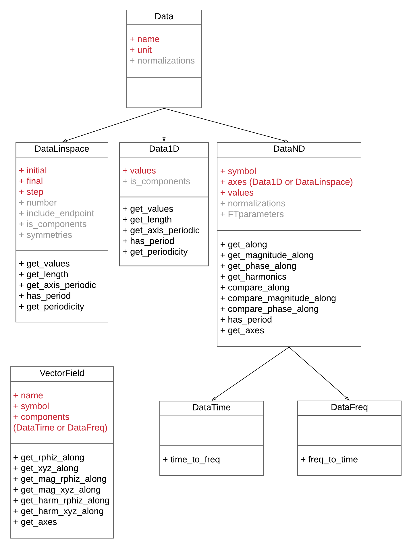
The attributes in red are mandatory, those in gray are optional. To correctly fill the mandatory attributes, it is advised to follow these principles:
valuesis a numpy arrayaxesis a list ofData1DorDataLinspacenameis string corresponding to a short description of the field, or thesymbolis a string giving the symbol of the field in LaTeX formatunitis a string among the list:[dimless, m, rad, °, g, s, min, h, Hz, rpm, degC, A, J, W, N, C, T, G, V, F, H, Ohm, At, Wb, Mx], with a prefix[k, h, da, d, c, m, etc.]. Composed units are also available (e.g.mm/s^2). It is best to use such a LaTeX formatting for axis labelling. Other units can be added in conversions.py.- for
Data1DandDataLinspace,name+[unit]can be used to label axes - for
DataTimeandDataFreq,namecan be used as plot title, andsymbol+[unit]as label
When a Data1D is created, the array values is squeezed to avoid dimension problems. When a DataTime or DataFreq is created, values is also squeezed, and a CheckDimError is raised if dimensions of axes and values do not match.
The following sections explain how to use the optional attributes to optimize storage.
2. How to reduce storage if an axis is regularly spaced
Axes often have a regular distribution, so that the use of DataLinspace allows to reduce the storage.
A DataLinspace object has five properties instead of the values array: initial, final, step and number allow to define the linspace vector (3 out of these 4 suffice), and include_endpoint is a boolean used to indicate whether the final point should be included or not (default False).
In the following example, the angle vector is defined as a linspace:
#---------------------------------------------------------------
# Create Data objects
Angle = DataLinspace(
    name="angle",
    unit="rad",
    initial=0,
    final=2*np.pi,
    number=20,
    include_endpoint=False,
)
print(Angle.get_values())
#---------------------------------------------------------------
[0.         0.31415927 0.62831853 0.9424778  1.25663706 1.57079633
 1.88495559 2.19911486 2.51327412 2.82743339 3.14159265 3.45575192
 3.76991118 4.08407045 4.39822972 4.71238898 5.02654825 5.34070751
 5.65486678 5.96902604]
3. How to reduce storage if a field presents a symmetry/periodicity
If a signal shows a symmetry or a periodicity along one or several of its axes, it is possible to store only the relevant part of the signal, and save the information necessary to rebuild it within the optional attribute symmetries. A repeting signal can either be periodic: $f(t+T)=f(t)$, or antiperiodic: $f(t+T)=-f(t)$. Indeed, we can consider that a symmetric signal is a periodic signal of period $T=N/2$.
symmetries is a dictionary containing the symmetry of the axis ({"period": n} or {"antiperiod": n}, with n the number of periods in the complete signal.
In the following example, the time vector and the field are reduced using the built-in method get_axis_periodic. To access the reconstructed axis values, the get_values method is available, with options to extract a single period or antiperiod:
Time_periodic = DataLinspace(
    name="time",
    unit="s",
    initial=0,
    final=5,
    number=5,
    include_endpoint=False,
    symmetries={"period": 6},
)
print(Time_periodic.get_values(is_oneperiod=True))
print(Time_periodic.get_values())
[0. 1. 2. 3. 4.]
[ 0.  1.  2.  3.  4.  5.  6.  7.  8.  9. 10. 11. 12. 13. 14. 15. 16. 17.
 18. 19. 20. 21. 22. 23. 24. 25. 26. 27. 28. 29.]
A special case can occur: when a single sample is periodic or antiperiodic. In this case, the distance between the points must be provided by the user:
Time_periodic = DataLinspace(
    name="time",
    unit="s",
    initial=0,
    final=0,
    number=1,
    include_endpoint=False,
    symmetries={"period": 6, "delta": 3},
)
print(Time_periodic.get_values(is_oneperiod=True))
print(Time_periodic.get_values())
[0.]
[ 0.  3.  6.  9. 12. 15.]
4. How to reduce storage if a field presents a pattern
If a signal shows a pattern (a repetition of certain slices) along one or several of its axes, it is also possible to reduce storage by storing only the unique slices. To do so, the DataPattern object can be used, with a rebuild_indices attribute which allows to reconstruct the whole field.
The whole axis (values_whole) must however also be provided since the rebuild indices are different between axis and field. It is also possible to store the indices which have been used to extract the unique slices in unique_indices; it is not used in SciDataTool but can be useful outside.
The slices can be either continuuous or by step, so that an is_step attribute has also been added (useful for field interpolations, integrations, etc).
Slices = DataPattern(
    name="z",
    unit="m",
    values=np.array([-5, -3, -1, 0]),
    values_whole=np.array([-5, -3, -3, -1, -1, 0, 1, 1, 3, 3, 5]),
    unique_indices=[0, 1, 3, 5],
    rebuild_indices=[0, 1, 1, 2, 2, 3, 2, 2, 1, 1, 0],
    is_step=True,
)
print(Slices.get_values(is_pattern=True))
print(Slices.get_values())
[-5 -3 -1  0]
[-5 -3 -3 -1 -1  0  1  1  3  3  5]
5. How to store a field in the frequency domain
If one prefers to store data in the frequency domain, for example because most postprocessings will handle spectra, or because a small number of harmonics allow to reduce storage, the DataFreq class can be used.
The definition is similar to the DataTime one, with the difference that the axes now have to be frequencies or wavenumbers and a DataFreq object is created.
Since we want to be able to go back to the time/space domain, there must exist a corresponding axis name. For the time being, the existing correspondances are:
"time"↔"freqs""angle"↔"wavenumber"
This list is to be expanded, and a possibility to manually add a correspondance will be implemented soon.
In the following example, a field is stored in a DataFreq object.
f = 50
freqs = np.array([-100, -50, 0, 50, 100])
Freqs = Data1D(name="freqs", unit="Hz", values=freqs)
field_ft = np.array(
    [
        0,
        3 + 5 * 1j,
        0,
        3 - 5 * 1j,
        0,
    ]
)
Field_FT = DataFreq(
    name="Example fft field",
    symbol="X_FT",
    axes=[Freqs],
    values=field_ft,
    unit="m",
)
A field can easily be transformed from time/space into Fourier domain, and vice-versa, using built-in methods:
Field = Field_FT.freq_to_time()
6. How to specify normalizations (axes or field)
If you plan to normalize your field or its axes during certain postprocessings (but not all), you might want to store the normalizations values. To do so, you can use the normalizations attribute, which is a dictionaray:
- for a normalization of the field, use
"ref"(e.g.{"ref": 0.8}) - for a normalization of an axis, use the name of the normalized axis unit (e.g.
{"elec_order": 60}) in the axis dict. There is no list of predefined normalized axis units, you simply must make sure to request it when you extract data (see How to extract slices) - to convert to a unit which does not exist in the predefined units, and if there exists a proportionality relation, it is also possible to add it in the
normalizationsdictionary (e.g.{"nameofmyunit": 154})
This dictionary can also be updated later.
See below examples of use of normalizations:
Time = Data1D(
    name="time",
    unit="s",
    values=time,
    normalizations={"elec_order": 3}
)

field = np.ones(10)
Field = DataTime(
    name="Example field",
    symbol="X",
    axes=[Time],
    values=field,
    normalizations={"ref": 10, "my_norm": 0.5}
)
normalizations can also contain an array, which should be the same size as the axis or the field, for non-linear normalizations. Normalization by a function is to be developed.
7. How to store a field with multiple components
It is more efficient to store all the components of a same field (e.g. $x$, $y$, $z$ components of a vector field, phases of a signal, etc.) in the same Data object. To do so, the is_components key can be used to easily recognize it, and strings can be used as values. In particular, using is_components ensures that no mathematical operation will be made on the axis values.
fieldA = np.ones(10)
fieldB = np.ones(10) * 5
fieldC = np.ones(10) * 10
new_field = np.array([field, fieldB, fieldC])

Phases = Data1D(name="phases", unit="", values=["Phase A","Phase B","Phase C"], is_components=True)
Field = DataTime(
    name="Example phase field",
    symbol="X",
    axes=[Phases, Time],
    values=new_field,
)
8. How to store a vector field
The VectorField class allows to store the vector components of a field (for example Fx, Fy, Fz for a force) into a single object. A VectorField object has a components attribute which is a dictionary of DataND objects. It has built-in methods to extract the components in cartesian or in polar coordinates.
Field_x = DataTime(
    name="Example field x",
    symbol="X_x",
    axes=[Time],
    values=fieldA,
)
Field_y = DataTime(
    name="Example field y",
    symbol="X_y",
    axes=[Time],
    values=fieldB,
)
Field_z = DataTime(
    name="Example field z",
    symbol="X_z",
    axes=[Time],
    values=fieldC,
)
VectField = VectorField(
    name="Example vector field",
    symbol="X",
    components={"comp_x": Field_x, "comp_y": Field_y, "comp_z": Field_z}
)
For cylindrical coordinates, the keys must be "radial", "tangential" and "axial".
Now that the Data objects have been created, we can: