Curved arch
April 2020, Amir Hossein Namadchi
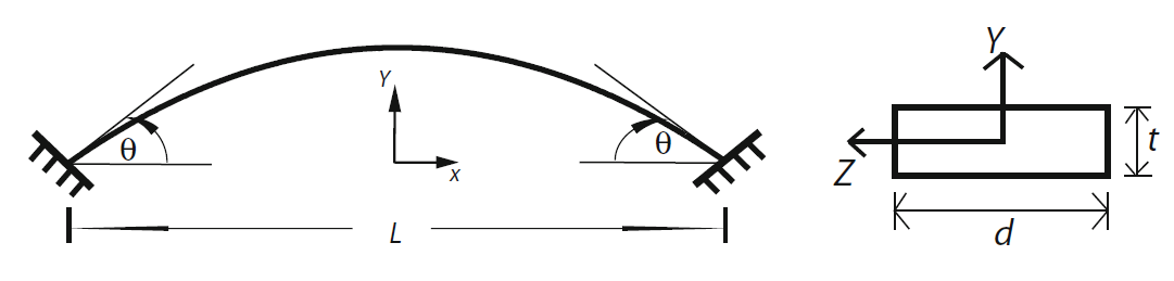
This is an OpenSeesPy simulation of one of the numerical examples in A robust composite time integration scheme for snap-through problems by Yenny Chandra et. al. It's a special problem involving dynamic snap-through with large deformations in elastic range. In their study, a new three sub-step composite time integration algorithm was presented to handle such problems. Here, I will use the Bathe scheme (TRBDF2) to perform transient analysis.
import numpy as np
import openseespy.opensees as ops
import matplotlib.pyplot as plt

from time import process_time
Below, the base units are defined as python variables:
# Units
mm = 1.0   # milimeters
N = 1.0    # Newtons
sec = 1.0  # Seconds
Model Defintion
# Node Coordinates Matrix (size : nn x 3)
node_coords = np.array([[-152.4, 0], [-137.337, 2.91714],
                        [-122.218, 5.53039], [-107.049, 7.8387],
                        [-91.8371, 9.84114], [-76.5878, 11.5369],
                        [-61.3076, 12.9252], [-46.0024, 14.0057],
                        [-30.6787, 14.7777], [-15.3424, 15.2411],
                        [0, 15.3955], [15.3424, 15.2411],
                        [30.6787, 14.7777], [46.0024, 14.0057],
                        [61.3076, 12.9252], [76.5878, 11.5369],
                        [91.8371, 9.84114], [107.049, 7.8387],
                        [122.218, 5.53039], [137.337, 2.91714],
                        [152.4, 0]], dtype = np.float64)*mm

# Element Connectivity Matrix (size: nel x 2)
connectivity = [[1, 2], [2, 3], [3, 4], [4, 5], [5, 6],
                [6, 7], [7, 8], [8, 9], [9, 10], [10, 11],
                [11, 12], [12, 13], [13, 14], [14, 15],
                [15, 16], [16, 17], [17, 18], [18, 19],
                [19, 20], [20, 21]]

# Get Number of total Nodes
nn = len(node_coords)
# Get Number of total Elements
nel = len(connectivity)

#Boundary Conditions (size: fixed_nodes x 4)
B_C = [[1,1,1,1],
       [nn,1,1,1]]


# Modulus of Elasticity
E = 206843*(N/mm**2)
# Mass Density
rho = (7.83e-9)*(N*(sec**2)/(mm**4))
# Cross-sectional area, 2nd Moment of Inertia
A, I_1 = (12.7*0.6096*mm*mm,
          (1/12)*(12.7*(0.6096**3))*mm**4)


ops.wipe()
ops.model('basic','-ndm',2,'-ndf',3)

# Adding nodes to the model object using list comprehensions
[ops.node(n+1,*node_coords[n]) for n in range(nn)];

# Applying BC
[ops.fix(B_C[n][0],*B_C[n][1:]) for n in range(len(B_C))];


#Set Transformation
ops.geomTransf('Corotational', 1)

# Adding Elements
[ops.element('elasticBeamColumn', e+1, *connectivity[e], A, E, I_1,1,
            '-mass',rho*A,'-cMass',1) for e in range(nel)];

# load function (Applied @ top node)
F = lambda t: (t if t<=8 else 8)*N

# Dynamic Analysis Parameters
dt = 0.0001
time = 15
time_domain = np.arange(0,time,dt)


# Loading Definition
ops.timeSeries('Path',1 , '-dt', dt,
               '-values', *np.vectorize(F)(time_domain),
               '-time', *time_domain)
ops.pattern('Plain', 1, 1)
ops.load(11, *[0.0, -1.0, 0.0])

# Analysis
ops.constraints('Transformation')
ops.numberer('RCM')
ops.system('ProfileSPD')
ops.test('NormUnbalance', 0.000001, 100)
ops.algorithm('Newton')
ops.integrator('TRBDF2')
ops.analysis('Transient')


# let's do this
time_lst =[]     # list to hold time stations for plotting
d_list = []      # list to hold vertical displacments of the top node

# start the timer
tic = process_time()

for i in range(len(time_domain)):
    ops.analyze(1, dt)
    time_lst.append(ops.getTime())
    d_list.append(ops.nodeDisp(11,2))

# stop the timer
toc = process_time()

print('Time elapsed:',toc-tic, 'sec')
Time elapsed: 29.2345874 sec
Visualization
plt.figure(figsize=(14,5))
ax1 = plt.axes()  # standard axes
plt.grid()
plt.yticks(fontname = 'Cambria', fontsize = 14)
plt.xticks(fontname = 'Cambria', fontsize = 14)
plt.title('Time history of vertical displacement of the top node',
          {'fontname':'Cambria',
           'fontstyle':'italic','size':18});

ax2 = plt.axes([0.65, 0.60, 0.2, 0.25])


ax1.plot(time_lst, d_list,'k')
ax2.plot(time_lst, d_list,'k')
ax2.set_xlim(left=13.5, right=14)
ax2.set_ylim(bottom=-15, top=-30)

ax1.set_xlabel('Time (sec)', {'fontname':'Cambria',
                            'fontstyle':'italic','size':14})
ax1.set_ylabel('Vertical Displacement (mm)', {'fontname':'Cambria',
                                 'fontstyle':'italic','size':14});

Closure
The figure deomnstrates a dynamic jump from the quasi static configuration. It then begins to oscillate around the remote equilibrium configuration. It is to be noted that conventional time integration algorithm like the Newmark method might not be able to present a stable and bounded solution like this. It is therefore necessary to employ an energy-conserving algorithms with proper numerical dissipation in order to tackle these kind of problems (like TRBDF2 and TRBDF3 in OpenSees).
References
Chandra, Y., Zhou, Y., Stanciulescu, I., Eason, T. and Spottswood, S., 2015. A robust composite time integration scheme for snap-through problems. Computational Mechanics, 55(5), pp.1041-1056.