https://www.coursera.org/learn/nlp-sequence-models
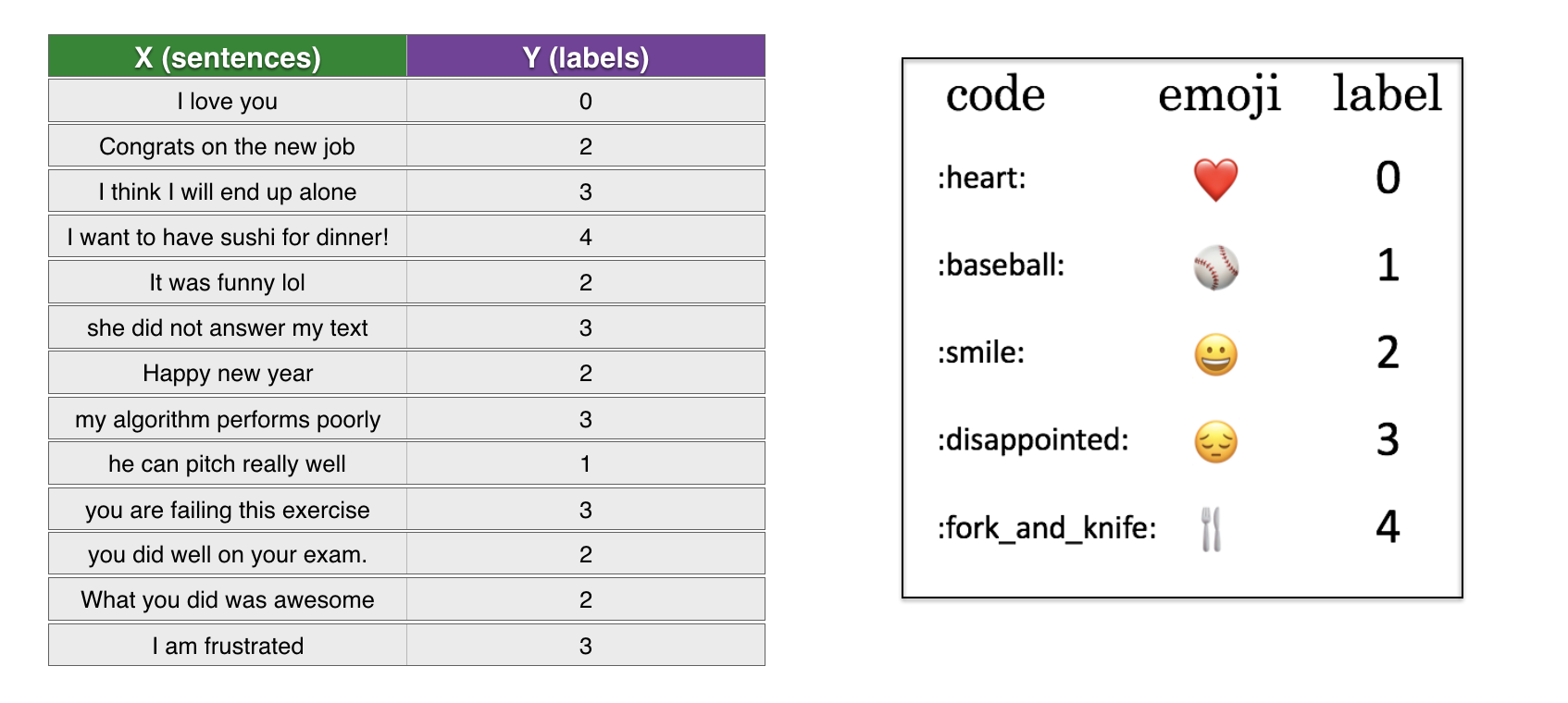
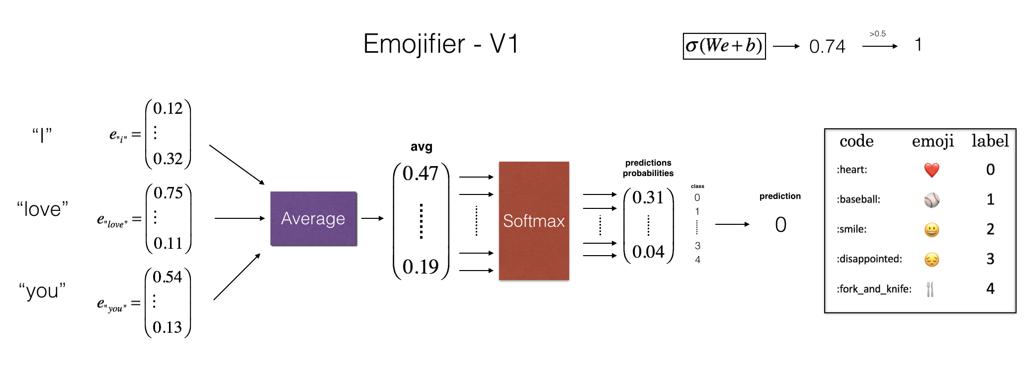
pip install emoji
import numpy as np
import matplotlib.pyplot as plt
import keras
%matplotlib inline
Using TensorFlow backend.
import csv
def read_csv(filename):
phrase = []
emoji = []
with open (filename) as csvDataFile:
csvReader = csv.reader(csvDataFile)
for row in csvReader:
phrase.append(row[0])
emoji.append(row[1])
X = np.asarray(phrase)
Y = np.asarray(emoji, dtype=int)
return X, Y
X_train, Y_train = read_csv('D:/dataset/NLP/emoji/train_emoji.csv')
X_test, Y_test = read_csv('D:/dataset/NLP/emoji/tesss.csv')
maxLen = len(max(X_train, key=len).split())
maxLen
10
import emoji
emoji_dictionary = {"0": "\u2764\uFE0F", # :heart: prints a black instead of red heart depending on the font
"1": ":baseball:",
"2": ":smile:",
"3": ":disappointed:",
"4": ":fork_and_knife:"}
def label_to_emoji(label):
return emoji.emojize(emoji_dictionary[str(label)], use_aliases=True)
index = 5
print(X_train[index], label_to_emoji(Y_train[index]))
I love you mum ❤️
Y_oh_train = keras.utils.to_categorical(Y_train, 5)
Y_oh_test = keras.utils.to_categorical(Y_test, 5)
index = 50
print(Y_train[index], "is converted into one hot", Y_oh_train[index])
0 is converted into one hot [1. 0. 0. 0. 0.]
As shown in Figure (2), the first step is to convert an input sentence into the word vector representation, which then get averaged together. Similar to the previous exercise, we will use pretrained 50-dimensional GloVe embeddings. Run the following cell to load the word_to_vec_map
, which contains all the vector representations.
def read_glove_vecs(glove_file):
with open(glove_file, encoding="utf8") as f:
words = set()
word_to_vec_map = {}
for line in f:
line = line.strip().split()
curr_word = line[0]
words.add(curr_word)
word_to_vec_map[curr_word] = np.array(line[1:], dtype=np.float64)
i = 1
words_to_index = {}
index_to_words = {}
for w in sorted(words):
words_to_index[w] = i
index_to_words[i] = w
i = i + 1
return words_to_index, index_to_words, word_to_vec_map
word_to_index, index_to_word, word_to_vec_map = read_glove_vecs('D:/dataset/glove.6B/glove.6B.50d.txt')
You've loaded:
word_to_index
: dictionary mapping from words to their indices in the vocabulary (400,001 words, with the valid indices ranging from 0 to 400,000)index_to_word
: dictionary mapping from indices to their corresponding words in the vocabularyword_to_vec_map
: dictionary mapping words to their GloVe vectorword = "ali"
index = 113317
print("the index of", word, "in the vocabulary is", word_to_index[word])
print("the", str(index) + "th word in the vocabulary is", index_to_word[index])
the index of ali in the vocabulary is 51314 the 113317th word in the vocabulary is cucumber
word_to_vec_map["ali"]
array([-0.71587 , 0.7874 , 0.71305 , -0.089955, 1.366 , -1.3149 , 0.7309 , 0.79725 , 0.47211 , 0.53347 , 0.37542 , -0.10256 , -1.0003 , -0.31226 , 0.26217 , 0.92426 , 0.43014 , -0.015593, 0.4149 , 0.88286 , 0.10869 , 0.95213 , 1.1807 , 0.06445 , -0.05814 , -1.797 , -0.18432 , -0.41754 , -0.73625 , 1.1607 , 1.5932 , -0.70268 , -0.61621 , 0.47118 , 0.95046 , 0.35206 , 0.6072 , 0.59339 , -0.47091 , 1.4916 , 0.27146 , 1.8252 , -1.2073 , -0.80058 , 0.52558 , -0.33346 , -1.4102 , -0.21514 , 0.12945 , -0.69603 ])
def sentence_to_avg(sentence, word_to_vec_map):
# Split sentence into list of lower case words
words = sentence.lower().split()
# Initialize the average word vector, should have the same shape as your word vectors.
avg = np.zeros((50,))
# average the word vectors. You can loop over the words in the list "words".
for w in words:
avg += word_to_vec_map[w]
avg = avg / len(words)
return avg
avg = sentence_to_avg("Morrocan couscous is my favorite dish", word_to_vec_map)
print("avg = ", avg)
avg = [-0.008005 0.56370833 -0.50427333 0.258865 0.55131103 0.03104983 -0.21013718 0.16893933 -0.09590267 0.141784 -0.15708967 0.18525867 0.6495785 0.38371117 0.21102167 0.11301667 0.02613967 0.26037767 0.05820667 -0.01578167 -0.12078833 -0.02471267 0.4128455 0.5152061 0.38756167 -0.898661 -0.535145 0.33501167 0.68806933 -0.2156265 1.797155 0.10476933 -0.36775333 0.750785 0.10282583 0.348925 -0.27262833 0.66768 -0.10706167 -0.283635 0.59580117 0.28747333 -0.3366635 0.23393817 0.34349183 0.178405 0.1166155 -0.076433 0.1445417 0.09808667]
Assuming here that $Yoh$ ("Y one hot") is the one-hot encoding of the output labels, the equations you need to implement in the forward pass and to compute the cross-entropy cost are: $$ z^{(i)} = W . avg^{(i)} + b$$ $$ a^{(i)} = softmax(z^{(i)})$$ $$ \mathcal{L}^{(i)} = - \sum_{k = 0}^{n_y - 1} Yoh^{(i)}_k * log(a^{(i)}_k)$$
It is possible to come up with a more efficient vectorized implementation. But since we are using a for-loop to convert the sentences one at a time into the avg^{(i)} representation anyway, let's not bother this time.
def softmax(x):
"""Compute softmax values for each sets of scores in x."""
e_x = np.exp(x - np.max(x))
return e_x / e_x.sum()
def predict(X, Y, W, b, word_to_vec_map):
"""
Given X (sentences) and Y (emoji indices), predict emojis and compute the accuracy of your model over the given set.
Arguments:
X -- input data containing sentences, numpy array of shape (m, None)
Y -- labels, containing index of the label emoji, numpy array of shape (m, 1)
Returns:
pred -- numpy array of shape (m, 1) with your predictions
"""
m = X.shape[0]
pred = np.zeros((m, 1))
for j in range(m): # Loop over training examples
# Split jth test example (sentence) into list of lower case words
words = X[j].lower().split()
# Average words' vectors
avg = np.zeros((50,))
for w in words:
avg += word_to_vec_map[w]
avg = avg/len(words)
# Forward propagation
Z = np.dot(W, avg) + b
A = softmax(Z)
pred[j] = np.argmax(A)
print("Accuracy: " + str(np.mean((pred[:] == Y.reshape(Y.shape[0],1)[:]))))
return pred
def model(X, Y, word_to_vec_map, learning_rate = 0.01, num_iterations = 401):
"""
Model to train word vector representations in numpy.
Arguments:
X -- input data, numpy array of sentences as strings, of shape (m, 1)
Y -- labels, numpy array of integers between 0 and 7, numpy-array of shape (m, 1)
word_to_vec_map -- dictionary mapping every word in a vocabulary into its 50-dimensional vector representation
learning_rate -- learning_rate for the stochastic gradient descent algorithm
num_iterations -- number of iterations
Returns:
pred -- vector of predictions, numpy-array of shape (m, 1)
W -- weight matrix of the softmax layer, of shape (n_y, n_h)
b -- bias of the softmax layer, of shape (n_y,)
"""
np.random.seed(1)
# Define number of training examples
m = Y.shape[0] # number of training examples
n_y = 5 # number of classes
n_h = 50 # dimensions of the GloVe vectors
# Initialize parameters using Xavier initialization
W = np.random.randn(n_y, n_h) / np.sqrt(n_h)
b = np.zeros((n_y,))
# Convert Y to Y_onehot with n_y classes
Y_oh = keras.utils.to_categorical(Y, n_y)
# Optimization loop
for t in range(num_iterations): # Loop over the number of iterations
for i in range(m): # Loop over the training examples
# Average the word vectors of the words from the i'th training example
avg = sentence_to_avg(X[i], word_to_vec_map)
# Forward propagate the avg through the softmax layer
z = np.dot(W, avg) + b
a = softmax(z)
# Compute cost using the i'th training label's one hot representation and "A" (the output of the softmax)
cost = -np.sum(Y_oh[i] * np.log(a))
# Compute gradients
dz = a - Y_oh[i]
dW = np.dot(dz.reshape(n_y,1), avg.reshape(1, n_h))
db = dz
# Update parameters with Stochastic Gradient Descent
W = W - learning_rate * dW
b = b - learning_rate * db
if t % 100 == 0:
print("Epoch: " + str(t) + " --- cost = " + str(cost))
pred = predict(X, Y, W, b, word_to_vec_map)
return pred, W, b
pred, W, b = model(X_train, Y_train, word_to_vec_map)
Epoch: 0 --- cost = 1.9520498812810072 Accuracy: 0.3484848484848485 Epoch: 100 --- cost = 0.07971818726014807 Accuracy: 0.9318181818181818 Epoch: 200 --- cost = 0.04456369243681402 Accuracy: 0.9545454545454546 Epoch: 300 --- cost = 0.03432267378786059 Accuracy: 0.9696969696969697 Epoch: 400 --- cost = 0.02906976783312465 Accuracy: 0.9772727272727273
print("Training set:")
pred_train = predict(X_train, Y_train, W, b, word_to_vec_map)
print('Test set:')
pred_test = predict(X_test, Y_test, W, b, word_to_vec_map)
Training set: Accuracy: 0.9772727272727273 Test set: Accuracy: 0.8571428571428571
Random guessing would have had 20% accuracy given that there are 5 classes. This is pretty good performance after training on only 127 examples.
In the training set, the algorithm saw the sentence "I love you" with the label ❤️. You can check however that the word "adore" does not appear in the training set. Nonetheless, lets see what happens if you write "I adore you."
def print_predictions(X, pred):
print()
for i in range(X.shape[0]):
print(X[i], label_to_emoji(int(pred[i])))
X_my_sentences = np.array(["i adore you", "i love you", "funny lol", "lets play with a ball", "food is ready", "not feeling happy"])
Y_my_labels = np.array([[0], [0], [2], [1], [4],[3]])
pred = predict(X_my_sentences, Y_my_labels , W, b, word_to_vec_map)
print_predictions(X_my_sentences, pred)
Accuracy: 0.8333333333333334 i adore you ❤️ i love you ❤️ funny lol 😄 lets play with a ball ⚾ food is ready 🍴 not feeling happy 😄
Amazing! Because adore has a similar embedding as love, the algorithm has generalized correctly even to a word it has never seen before. Words such as heart, dear, beloved or adore have embedding vectors similar to love, and so might work too---feel free to modify the inputs above and try out a variety of input sentences. How well does it work?
Note though that it doesn't get "not feeling happy" correct. This algorithm ignores word ordering, so is not good at understanding phrases like "not happy."
Printing the confusion matrix can also help understand which classes are more difficult for your model. A confusion matrix shows how often an example whose label is one class ("actual" class) is mislabeled by the algorithm with a different class ("predicted" class).
Let's build an LSTM model that takes as input word sequences. This model will be able to take word ordering into account. Emojifier-V2 will continue to use pre-trained word embeddings to represent words, but will feed them into an LSTM, whose job it is to predict the most appropriate emoji.
Run the following cell to load the Keras packages.
import numpy as np
np.random.seed(0)
from keras.models import Model
from keras.layers import Dense, Input, Dropout, LSTM, Activation
from keras.layers.embeddings import Embedding
from keras.preprocessing import sequence
from keras.initializers import glorot_uniform
np.random.seed(1)
Here is the Emojifier-v2 you will implement:
In Keras, the embedding matrix is represented as a "layer", and maps positive integers (indices corresponding to words) into dense vectors of fixed size (the embedding vectors). It can be trained or initialized with a pretrained embedding. In this part, you will learn how to create an Embedding() layer in Keras, initialize it with the GloVe 50-dimensional vectors loaded earlier in the notebook. Because our training set is quite small, we will not update the word embeddings but will instead leave their values fixed. But in the code below, we'll show you how Keras allows you to either train or leave fixed this layer.
The Embedding()
layer takes an integer matrix of size (batch size, max input length) as input. This corresponds to sentences converted into lists of indices (integers), as shown in the figure below.
The largest integer (i.e. word index) in the input should be no larger than the vocabulary size. The layer outputs an array of shape (batch size, max input length, dimension of word vectors).
The first step is to convert all your training sentences into lists of indices, and then zero-pad all these lists so that their length is the length of the longest sentence.
def sentences_to_indices(X, word_to_index, max_len):
m = X.shape[0] # number of training examples
# Initialize X_indices as a numpy matrix of zeros and the correct shape (≈ 1 line)
X_indices = np.zeros((m, max_len))
for i in range(m): # loop over training examples
# Convert the ith training sentence in lower case and split is into words. You should get a list of words.
sentence_words =X[i].lower().split()
# Loop over the words of sentence_words
for j, w in enumerate(sentence_words):
# Set the (i,j)th entry of X_indices to the index of the correct word.
X_indices[i, j] = word_to_index[w]
return X_indices
Run the following cell to check what sentences_to_indices()
does, and check your results.
X1 = np.array(["funny lol", "lets play baseball", "food is ready for you"])
X1_indices = sentences_to_indices(X1,word_to_index, max_len = 5)
print("X1 =", X1)
print("X1_indices =", X1_indices)
X1 = ['funny lol' 'lets play baseball' 'food is ready for you'] X1_indices = [[155345. 225122. 0. 0. 0.] [220930. 286375. 69714. 0. 0.] [151204. 192973. 302254. 151349. 394475.]]
Let's build the Embedding()
layer in Keras, using pre-trained word vectors. After this layer is built, you will pass the output of sentences_to_indices()
to it as an input, and the Embedding()
layer will return the word embeddings for a sentence.
word_to_vec_map
.trainable = False
when calling Embedding()
. If you were to set trainable = True
, then it will allow the optimization algorithm to modify the values of the word embeddings.from keras.layers import Embedding
def pretrained_embedding_layer(word_to_vec_map, word_to_index):
vocab_len = len(word_to_index) + 1 # adding 1 to fit Keras embedding (requirement)
emb_dim = word_to_vec_map["cucumber"].shape[0] # define dimensionality of your GloVe word vectors (= 50)
# Initialize the embedding matrix as a numpy array of zeros of shape (vocab_len, dimensions of word vectors = emb_dim)
emb_matrix = np.zeros((vocab_len, emb_dim))
# Set each row "index" of the embedding matrix to be the word vector representation of the "index"th word of the vocabulary
for word, index in word_to_index.items():
emb_matrix[index, :] = word_to_vec_map[word]
# Define Keras embedding layer with the correct output/input sizes, make it trainable. Use Embedding(...). Make sure to set trainable=False.
embedding_layer = Embedding(vocab_len, emb_dim, trainable = False)
# Build the embedding layer, it is required before setting the weights of the embedding layer. Do not modify the "None".
embedding_layer.build((None,))
# Set the weights of the embedding layer to the embedding matrix. Your layer is now pretrained.
embedding_layer.set_weights([emb_matrix])
return embedding_layer
from keras.layers import Input
from keras.layers import LSTM
from keras.layers import Dense, Dropout
from keras.models import Model
def Emojify_V2(input_shape, word_to_vec_map, word_to_index):
# Define sentence_indices as the input of the graph, it should be of shape input_shape and dtype 'int32' (as it contains indices).
sentence_indices = Input(input_shape, dtype = np.int32)
# Create the embedding layer pretrained with GloVe Vectors (≈1 line)
embedding_layer = pretrained_embedding_layer(word_to_vec_map, word_to_index)
# Propagate sentence_indices through your embedding layer, you get back the embeddings
embeddings = embedding_layer(sentence_indices)
# Propagate the embeddings through an LSTM layer with 128-dimensional hidden state
# Be careful, the returned output should be a batch of sequences.
X = LSTM(128, return_sequences=True)(embeddings)
# Add dropout with a probability of 0.5
X = Dropout(0.5)(X)
# Propagate X trough another LSTM layer with 128-dimensional hidden state
# Be careful, the returned output should be a single hidden state, not a batch of sequences.
X = LSTM(128)(X)
# Add dropout with a probability of 0.5
X = Dropout(0.5)(X)
# Propagate X through a Dense layer with softmax activation to get back a batch of 5-dimensional vectors.
X = Dense(5, activation = 'softmax')(X)
# Create Model instance which converts sentence_indices into X.
model = Model(sentence_indices, X)
return model
model = Emojify_V2((maxLen,), word_to_vec_map, word_to_index)
model.summary()
Model: "model_1" _________________________________________________________________ Layer (type) Output Shape Param # ================================================================= input_2 (InputLayer) (None, 10) 0 _________________________________________________________________ embedding_2 (Embedding) (None, 10, 50) 20000050 _________________________________________________________________ lstm_3 (LSTM) (None, 10, 128) 91648 _________________________________________________________________ dropout_3 (Dropout) (None, 10, 128) 0 _________________________________________________________________ lstm_4 (LSTM) (None, 128) 131584 _________________________________________________________________ dropout_4 (Dropout) (None, 128) 0 _________________________________________________________________ dense_2 (Dense) (None, 5) 645 ================================================================= Total params: 20,223,927 Trainable params: 223,877 Non-trainable params: 20,000,050 _________________________________________________________________
As usual, after creating your model in Keras, you need to compile it and define what loss, optimizer and metrics your are want to use. Compile your model using categorical_crossentropy
loss, adam
optimizer and ['accuracy']
metrics:
model.compile(loss='categorical_crossentropy', optimizer='adam', metrics=['accuracy'])
It's time to train your model. Your Emojifier-V2 model
takes as input an array of shape (m
, max_len
) and outputs probability vectors of shape (m
, number of classes
). We thus have to convert X_train (array of sentences as strings) to X_train_indices (array of sentences as list of word indices), and Y_train (labels as indices) to Y_train_oh (labels as one-hot vectors).
X_train_indices = sentences_to_indices(X_train, word_to_index, maxLen)
Y_train_oh = keras.utils.to_categorical(Y_train, 5)
model.fit(X_train_indices, Y_train_oh, epochs = 50, batch_size = 32, shuffle=True)
Epoch 1/50 132/132 [==============================] - 2s 14ms/step - loss: 1.5785 - accuracy: 0.2803 Epoch 2/50 132/132 [==============================] - 0s 2ms/step - loss: 1.5018 - accuracy: 0.3333 Epoch 3/50 132/132 [==============================] - 0s 2ms/step - loss: 1.4604 - accuracy: 0.3485 Epoch 4/50 132/132 [==============================] - 0s 2ms/step - loss: 1.3685 - accuracy: 0.4470 Epoch 5/50 132/132 [==============================] - 0s 2ms/step - loss: 1.2991 - accuracy: 0.4697 Epoch 6/50 132/132 [==============================] - 0s 2ms/step - loss: 1.1840 - accuracy: 0.5455 Epoch 7/50 132/132 [==============================] - 0s 2ms/step - loss: 1.0434 - accuracy: 0.6061 Epoch 8/50 132/132 [==============================] - 0s 2ms/step - loss: 0.8732 - accuracy: 0.7197 Epoch 9/50 132/132 [==============================] - 0s 2ms/step - loss: 0.8077 - accuracy: 0.7273 Epoch 10/50 132/132 [==============================] - 0s 2ms/step - loss: 0.6823 - accuracy: 0.7500 Epoch 11/50 132/132 [==============================] - 0s 2ms/step - loss: 0.6593 - accuracy: 0.7424 Epoch 12/50 132/132 [==============================] - 0s 2ms/step - loss: 0.5245 - accuracy: 0.7879 Epoch 13/50 132/132 [==============================] - 0s 2ms/step - loss: 0.5793 - accuracy: 0.8106 Epoch 14/50 132/132 [==============================] - 0s 2ms/step - loss: 0.4114 - accuracy: 0.8712 Epoch 15/50 132/132 [==============================] - 0s 2ms/step - loss: 0.4243 - accuracy: 0.8333 Epoch 16/50 132/132 [==============================] - 0s 2ms/step - loss: 0.3319 - accuracy: 0.8788 Epoch 17/50 132/132 [==============================] - 0s 2ms/step - loss: 0.3110 - accuracy: 0.8864 Epoch 18/50 132/132 [==============================] - 0s 2ms/step - loss: 0.3255 - accuracy: 0.8864 Epoch 19/50 132/132 [==============================] - 0s 2ms/step - loss: 0.3134 - accuracy: 0.9167 Epoch 20/50 132/132 [==============================] - 0s 2ms/step - loss: 0.2598 - accuracy: 0.9015 Epoch 21/50 132/132 [==============================] - 0s 2ms/step - loss: 0.2034 - accuracy: 0.9318 Epoch 22/50 132/132 [==============================] - 0s 2ms/step - loss: 0.3006 - accuracy: 0.8939 Epoch 23/50 132/132 [==============================] - 0s 2ms/step - loss: 0.1704 - accuracy: 0.9394 Epoch 24/50 132/132 [==============================] - 0s 2ms/step - loss: 0.1986 - accuracy: 0.9470 Epoch 25/50 132/132 [==============================] - 0s 2ms/step - loss: 0.1613 - accuracy: 0.9621 Epoch 26/50 132/132 [==============================] - 0s 2ms/step - loss: 0.1410 - accuracy: 0.9545 Epoch 27/50 132/132 [==============================] - 0s 2ms/step - loss: 0.1857 - accuracy: 0.9167 Epoch 28/50 132/132 [==============================] - 0s 2ms/step - loss: 0.2262 - accuracy: 0.9394 Epoch 29/50 132/132 [==============================] - 0s 2ms/step - loss: 0.1146 - accuracy: 0.9470 Epoch 30/50 132/132 [==============================] - 0s 2ms/step - loss: 0.1039 - accuracy: 0.9697 Epoch 31/50 132/132 [==============================] - 0s 2ms/step - loss: 0.1061 - accuracy: 0.9621 Epoch 32/50 132/132 [==============================] - 0s 2ms/step - loss: 0.2473 - accuracy: 0.9167 Epoch 33/50 132/132 [==============================] - 0s 2ms/step - loss: 0.1782 - accuracy: 0.9318 Epoch 34/50 132/132 [==============================] - 0s 2ms/step - loss: 0.1944 - accuracy: 0.9394 Epoch 35/50 132/132 [==============================] - 0s 2ms/step - loss: 0.1595 - accuracy: 0.9318 Epoch 36/50 132/132 [==============================] - 0s 2ms/step - loss: 0.1048 - accuracy: 0.9545 Epoch 37/50 132/132 [==============================] - 0s 2ms/step - loss: 0.1591 - accuracy: 0.9545 Epoch 38/50 132/132 [==============================] - 0s 2ms/step - loss: 0.0960 - accuracy: 0.9621 Epoch 39/50 132/132 [==============================] - 0s 2ms/step - loss: 0.0617 - accuracy: 0.9924 Epoch 40/50 132/132 [==============================] - 0s 2ms/step - loss: 0.0381 - accuracy: 1.0000 Epoch 41/50 132/132 [==============================] - 0s 2ms/step - loss: 0.0345 - accuracy: 1.0000 Epoch 42/50 132/132 [==============================] - 0s 2ms/step - loss: 0.0371 - accuracy: 1.0000 Epoch 43/50 132/132 [==============================] - 0s 2ms/step - loss: 0.1414 - accuracy: 0.9621 Epoch 44/50 132/132 [==============================] - 0s 2ms/step - loss: 0.0375 - accuracy: 0.9924 Epoch 45/50 132/132 [==============================] - 0s 2ms/step - loss: 0.0719 - accuracy: 0.9848 Epoch 46/50 132/132 [==============================] - 0s 2ms/step - loss: 0.0595 - accuracy: 0.9848 Epoch 47/50 132/132 [==============================] - 0s 2ms/step - loss: 0.0240 - accuracy: 0.9848 Epoch 48/50 132/132 [==============================] - 0s 2ms/step - loss: 0.0170 - accuracy: 1.0000 Epoch 49/50 132/132 [==============================] - 0s 2ms/step - loss: 0.0152 - accuracy: 1.0000 Epoch 50/50 132/132 [==============================] - 0s 2ms/step - loss: 0.0097 - accuracy: 1.0000
<keras.callbacks.callbacks.History at 0x1ef0b539e80>
Your model should perform close to 100% accuracy on the training set. The exact accuracy you get may be a little different. Run the following cell to evaluate your model on the test set.
X_test_indices = sentences_to_indices(X_test, word_to_index, max_len = maxLen)
Y_test_oh = keras.utils.to_categorical(Y_test, 5)
loss, acc = model.evaluate(X_test_indices, Y_test_oh)
print()
print("Test accuracy = ", acc)
56/56 [==============================] - 0s 4ms/step Test accuracy = 0.8035714030265808
You should get a test accuracy between 80% and 95%. Run the cell below to see the mislabelled examples.
# This code allows you to see the mislabelled examples
C = 5
y_test_oh = np.eye(C)[Y_test.reshape(-1)]
X_test_indices = sentences_to_indices(X_test, word_to_index, maxLen)
pred = model.predict(X_test_indices)
for i in range(len(X_test)):
x = X_test_indices
num = np.argmax(pred[i])
if(num != Y_test[i]):
print('Expected emoji:'+ label_to_emoji(Y_test[i]) + ' prediction: '+ X_test[i] + label_to_emoji(num).strip())
Expected emoji:😄 prediction: she got me a nice present ❤️ Expected emoji:😞 prediction: work is hard 😄 Expected emoji:😞 prediction: This girl is messing with me ❤️ Expected emoji:😞 prediction: work is horrible 😄 Expected emoji:🍴 prediction: any suggestions for dinner 😄 Expected emoji:😄 prediction: you brighten my day ❤️ Expected emoji:😞 prediction: she is a bully ❤️ Expected emoji:😞 prediction: My life is so boring ❤️ Expected emoji:😄 prediction: What you did was awesome 😞 Expected emoji:😞 prediction: go away ⚾ Expected emoji:❤️ prediction: family is all I have 😞
Now you can try it on your own example. Write your own sentence below.
# Change the sentence below to see your prediction. Make sure all the words are in the Glove embeddings.
x_test = np.array(['not feeling happy'])
X_test_indices = sentences_to_indices(x_test, word_to_index, maxLen)
print(x_test[0] +' '+ label_to_emoji(np.argmax(model.predict(X_test_indices))))
not feeling happy 😞
Previously, Emojify-V1 model did not correctly label "not feeling happy," but our implementation of Emojiy-V2 got it right. (Keras' outputs are slightly random each time, so you may not have obtained the same result.) The current model still isn't very robust at understanding negation (like "not happy") because the training set is small and so doesn't have a lot of examples of negation. But if the training set were larger, the LSTM model would be much better than the Emojify-V1 model at understanding such complex sentences.