
Flood Mapping from Single Sentinel-1 SAR Images

Franz J Meyer, University of Alaska Fairbanks
This notebook presents a SAR-based flood mapping approach that largely follows a methodology developed by the German Aerospace Center and published in Sentinel-1-based flood mapping: a fully automated processing chain by Twele et al.. The approach is based on radiometricall terrain corrected (RTC processed) Sentinel-1 SAR data and applies a dynamic thresholding method followed by fuzzy-logic-based post processing procedure. This notebook implements the initial threshold-based flood mapping approach but, for simplicity, does not include the fuzzy-logic post processing steps.
The approach is based on image amplitude data and is capable of detecting standing surface water. Note that flooding under vegetation will not be detected by this approach.
Important Notes about Binder
The Binder server will automatically shutdown when left idle for more than 10 minutes. Your notebook edits will be lost when this happens. You will need to relaunch the binder to continue working in a fresh copy of the notebook.
How to Save your Notebook Edits
The Easy Way
Click on the Jupyter logo at the top left of the screen to access the file manager. Download the notebook, then upload and run it the next time you restart the server.
The Better, More Complicated Way
This solution requires some knowledge of git. Fork the asf-jupyter-notebook repository and update the url for the Binder launch button to the url of your fork. The url to edit can be found in the first line of the README.md file for this branch. Once you have your own fork, push any notebook changes to it prior to shutting down the server or allowing it to time out.
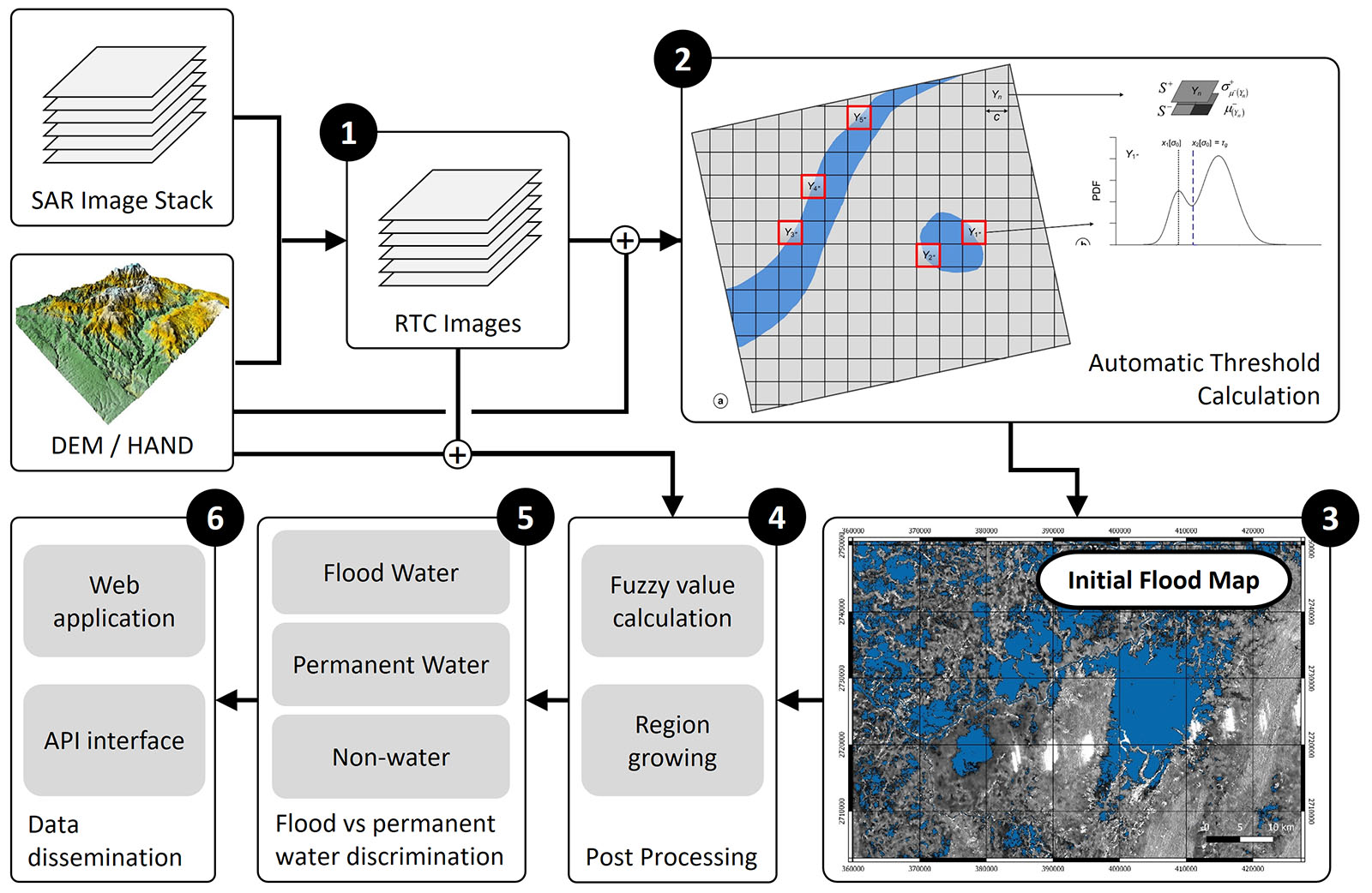
General Methodology and Workflow
The workflow of the Sentinel-1-based processing chain, as outlined in the figure below, is composed of the following main elements:
- Find relevant SAR data over your area of interest at the Alaska Satellite Facility's SAR archive and Perform geometric and radiometric terrain correction using the RTC processing flow by GAMMA Remote Sensing,
- adaptive and automatic threshold calculation as discussed in the course,
- initial flood detection by applying the calculated threshold image wide,
- fuzzy-logic-based classification refinement,
- final classification into permanent and flood waters using auxiliary data, and
- dissemination of the results.
Step 1 of this workflow are operationally implemented in the Alaska Satellite Facility's Hybrid Pluggable Processing Pipeline (HyP3) environment and accessible to the public at the HyP3 Website. This notebook will focus on Steps 2 and 3
Flood Mapping Procedure
Loading Python Libraries
import glob
import os
from typing import Tuple

import numpy as np
from osgeo import gdal
import pyproj
import pandas as pd
import rasterio
import skfuzzy

import ipywidgets as ui

import matplotlib.pyplot as plt # for add_subplot, axis, figure, imshow, legend, plot, set_axis_off, set_data,
                                # set_title, set_xlabel, set_ylabel, set_ylim, subplots, title, twinx

from asf_notebook_FloodMapping import handle_old_data
from asf_notebook_FloodMapping import input_path
from asf_notebook_FloodMapping import NoHANDLayerException

%matplotlib widget
Write Some Helper Scripts
Write a function to pad an image, so it may be split into tiles with consistent dimensions
def pad_image(image: np.ndarray, to: int) -> np.ndarray:
    height, width = image.shape

    n_rows, n_cols = get_tile_row_col_count(height, width, to)
    new_height = n_rows * to
    new_width = n_cols * to

    padded = np.zeros((new_height, new_width))
    padded[:image.shape[0], :image.shape[1]] = image
    return padded
Write a function to tile an image
#def tile_image(image: np.ndarray, width: int = 200, height: int = 200) -> np.ndarray:
def tile_image(image: np.ndarray, width, height) -> np.ndarray:
    _nrows, _ncols = image.shape
    _strides = image.strides

    nrows, _m = divmod(_nrows, height)
    ncols, _n = divmod(_ncols, width)

    assert _m == 0, "Image must be evenly tileable. Please pad it first"
    assert _n == 0, "Image must be evenly tileable. Please pad it first"

    return np.lib.stride_tricks.as_strided(
        np.ravel(image),
        shape=(nrows, ncols, height, width),
        strides=(height * _strides[0], width * _strides[1], *_strides),
        writeable=False
    ).reshape(nrows * ncols, height, width)
Write a function for multi-class Expectation Maximization Thresholding
def EMSeg_opt(image, number_of_classes):
    image_copy = image.copy()
    image_copy2 = np.ma.filled(image.astype(float), np.nan) # needed for valid posterior_lookup keys
    image = image.flatten()
    minimum = np.amin(image)
    image = image - minimum + 1
    maximum = np.amax(image)

    size = image.size
    histogram = make_histogram(image)
    nonzero_indices = np.nonzero(histogram)[0]
    histogram = histogram[nonzero_indices]
    histogram = histogram.flatten()
    class_means = (
            (np.arange(number_of_classes) + 1) * maximum /
            (number_of_classes + 1)
    )
    class_variances = np.ones((number_of_classes)) * maximum
    class_proportions = np.ones((number_of_classes)) * 1 / number_of_classes
    sml = np.mean(np.diff(nonzero_indices)) / 1000
    iteration = 0
    while(True):
        class_likelihood = make_distribution(
            class_means, class_variances, class_proportions, nonzero_indices
        )
        sum_likelihood = np.sum(class_likelihood, 1) + np.finfo(
                class_likelihood[0][0]).eps
        log_likelihood = np.sum(histogram * np.log(sum_likelihood))
        for j in range(0, number_of_classes):
            class_posterior_probability = (
                histogram * class_likelihood[:,j] / sum_likelihood
            )
            class_proportions[j] = np.sum(class_posterior_probability)
            class_means[j] = (
                np.sum(nonzero_indices * class_posterior_probability)
                    / class_proportions[j]
            )
            vr = (nonzero_indices - class_means[j])
            class_variances[j] = (
                np.sum(vr *vr * class_posterior_probability)
                    / class_proportions[j] +sml
            )
            del class_posterior_probability, vr
        class_proportions = class_proportions + 1e-3
        class_proportions = class_proportions / np.sum(class_proportions)
        class_likelihood = make_distribution(
            class_means, class_variances, class_proportions, nonzero_indices
        )
        sum_likelihood = np.sum(class_likelihood, 1) + np.finfo(
                class_likelihood[0,0]).eps
        del class_likelihood
        new_log_likelihood = np.sum(histogram * np.log(sum_likelihood))
        del sum_likelihood
        if((new_log_likelihood - log_likelihood) < 0.000001):
            break
        iteration = iteration + 1
    del log_likelihood, new_log_likelihood
    class_means = class_means + minimum - 1
    s = image_copy.shape
    posterior = np.zeros((s[0], s[1], number_of_classes))
    posterior_lookup = dict()
    for i in range(0, s[0]):
        for j in range(0, s[1]):
            pixel_val = image_copy2[i,j]
            if pixel_val in posterior_lookup:
                for n in range(0, number_of_classes):
                    posterior[i,j,n] = posterior_lookup[pixel_val][n]
            else:
                posterior_lookup.update({pixel_val: [0]*number_of_classes})
                for n in range(0, number_of_classes):
                    x = make_distribution(
                        class_means[n], class_variances[n], class_proportions[n],
                        image_copy[i,j]
                    )
                    posterior[i,j,n] = x * class_proportions[n]
                    posterior_lookup[pixel_val][n] = posterior[i,j,n]
    return posterior, class_means, class_variances, class_proportions

def make_histogram(image):
    image = image.flatten()
    indices = np.nonzero(np.isnan(image))
    image[indices] = 0
    indices = np.nonzero(np.isinf(image))
    image[indices] = 0
    del indices
    size = image.size
    maximum = int(np.ceil(np.amax(image)) + 1)
    #maximum = (np.ceil(np.amax(image)) + 1)
    histogram = np.zeros((1, maximum))
    for i in range(0,size):
        #floor_value = int(np.floor(image[i]))
        floor_value = np.floor(image[i]).astype(np.uint8)
        #floor_value = (np.floor(image[i]))
        if floor_value > 0 and floor_value < maximum - 1:
            temp1 = image[i] - floor_value
            temp2 = 1 - temp1
            histogram[0,floor_value] = histogram[0,floor_value] + temp1
            histogram[0,floor_value - 1] = histogram[0,floor_value - 1] + temp2
    histogram = np.convolve(histogram[0], [1,2,3,2,1])
    histogram = histogram[2:(histogram.size - 3)]
    histogram = histogram / np.sum(histogram)
    return histogram

def make_distribution(m, v, g, x):
    x = x.flatten()
    m = m.flatten()
    v = v.flatten()
    g = g.flatten()
    y = np.zeros((len(x), m.shape[0]))
    for i in range(0,m.shape[0]):
        d = x - m[i]
        amp = g[i] / np.sqrt(2*np.pi*v[i])
        y[:,i] = amp * np.exp(-0.5 * (d * d) / v[i])
    return y

def get_proj4(filename):
    f=rasterio.open(filename)
    return pyproj.Proj(f.crs, preserve_units=True)  #used in pysheds

def gdal_read(filename, ndtype=np.float64):
    '''
    z=readData('/path/to/file')
    '''
    ds = gdal.Open(filename)
    return np.array(ds.GetRasterBand(1).ReadAsArray()).astype(ndtype);
def gdal_get_geotransform(filename):
    '''
    [top left x, w-e pixel resolution, rotation, top left y, rotation, n-s pixel resolution]=gdal_get_geotransform('/path/to/file')
    '''
    #http://stackoverflow.com/questions/2922532/obtain-latitude-and-longitude-from-a-geotiff-file
    ds = gdal.Open(filename)
    return ds.GetGeoTransform()
Write a function to calculate the number of rows and columns of tiles needed to tile an image to a given size
def get_tile_row_col_count(height: int, width: int, tile_size: int) -> Tuple[int, int]:
    return int(np.ceil(height / tile_size)), int(np.ceil(width / tile_size))
Write a function to extract the tiff dates from a wildcard path:
def get_dates(paths):
    dates = []
    pths = glob.glob(paths)
    for p in pths:
        date = p.split('/')[-1].split("_")[0]
        dates.append(date)
    dates.sort()
    return dates
Write a function to save a mask
def write_mask_to_file(mask: np.ndarray, file_name: str, projection: str, geo_transform: str) -> None:
    (width, height) = mask.shape
    out_image = gdal.GetDriverByName('GTiff').Create(
        file_name, height, width, bands=1
    )
    out_image.SetProjection(projection)
    out_image.SetGeoTransform(geo_transform)
    out_image.GetRasterBand(1).WriteArray(mask)
    out_image.GetRasterBand(1).SetNoDataValue(0)
    out_image.FlushCache()
Load SAR Data Sets to Process
def get_tiff_paths(paths: str) -> list:
    tiff_paths = !ls $paths | sort -t_ -k5,5
    return tiff_paths
Reading a SAR Data Stack:
This lab uses a subset of a Sentinel-1 SAR time series acquired near the city of Malda, on the Indian Bangladesh border. This area experienced extensive flooding during the 2020 South Asia monsoon season. The time series covers June to August of 2020 and combines ascending and descending RTC imagery into a joint and consistent time series to monitoring this rapidly developing event.
name = "BangladeshFloodMapping_binder"
tiff_dir = path = f"/home/jovyan/{name}"
if not os.path.exists(tiff_dir):
    os.mkdir(tiff_dir)
os.chdir(tiff_dir)
print(f"Current working directory: {os.getcwd()}")

time_series_path = f"s3://asf-jupyter-data-west/{name}.tar.gz"
time_series = os.path.basename(time_series_path)
!aws --no-sign-request --region us-west-2 s3 cp $time_series_path $time_series

!tar -xvzf {name}.tar.gz
!rm *.tar.gz
Move into the parent directory of the directory containing the data and create a directory in which to store the water masks
analysis_directory = tiff_dir
os.chdir(tiff_dir)
mask_directory = f'{analysis_directory}/Water_Masks'
if not os.path.exists(mask_directory):
    os.mkdir(mask_directory)
print(f"Current working directory: {os.getcwd()}")

paths = f"{tiff_dir}/*_V*.tif*"
if os.path.exists(tiff_dir):
    tiff_paths = get_tiff_paths(paths)
Write a function to create a dictionary containing lists of each vv/vh pair
def group_polarizations(tiff_paths: list) -> dict:
    pths = {}
    for tiff in tiff_paths:
        product_name = tiff.split('.')[0][:-2]
        if product_name in pths:
            pths[product_name].append(tiff)
        else:
            pths.update({product_name: [tiff]})
            pths[product_name].sort()
    return pths
Write a function to confirm the presence of both VV and VH images in all image sets
def confirm_dual_polarizations(paths: dict) -> bool:
    for p in paths:
        if len(paths[p]) == 2:
            if ('vv' not in paths[p][1] and 'VV' not in paths[p][1]) or \
            ('vh' not in paths[p][0] and 'VH' not in paths[p][0]):
                return False
    return True
Create a dictionary of VV/VH pairs and check it for completeness
grouped_pths = group_polarizations(tiff_paths)
if not confirm_dual_polarizations(grouped_pths):
    print("ERROR: AI_Water requires both VV and VH polarizations.")
else:
    print("Confirmed presence of VV and VH polarities for each product.")

#print(grouped_pths) #uncomment to print VV/VH path pairs
Load HAND Layer for your AOI and Create HAND-Exclusion Mask (HAND-EM)
This notebook uses a prepared Height Above Nearest Drainage (HAND) file that was cut to the same extent as the SAR image time series. A DEM is used to create HAND by calculating the height difference between a particular image pixels and the nearest drainage (such as the nearest river).
To create the HAND Exclusion Mask (HAND-EM) we then threshold the HAND layer by assuming that pixels with a HAND value > 15 m are unlikely to be flooded. This means, in other words, we assume that flood waters are unlikely to exceed a depth of 15 m.
#load HAND and derive HAND-EM
Hthresh = 15

HAND_file="/home/jovyan/BangladeshFloodMapping_binder/Bangladesh_Training_DEM_hand.tif"
print(f"Selected HAND: {HAND_file}")
try:
    HAND_gT=gdal_get_geotransform(HAND_file)
except AttributeError:
    raise NoHANDLayerException("Remember to select a HAND layer in the previous cell.")
HAND_proj4=get_proj4(HAND_file)
HAND=gdal_read(HAND_file)
hand = np.nan_to_num(HAND)

# Create Binary HAND-EM
Hmask = hand < Hthresh
handem = np.zeros_like(hand)
sel = np.ones_like(hand)
handem[Hmask] = sel[Hmask]
Now let's plot HAND and HAND-EM side-by-side. Dark blue regions in the HAND file (left) area areas near drainage systems such as rivers. These areas are most likely to be affected by floods. Areas in red, however, are at higher elevations and less likely to be flooded.
The HAND-EM layer to the right shows pixels unlikely to contain flood waters in black. These pixels are at least 15 m above the nearest drainage system.
fig = plt.figure(figsize=(9, 5))
plt.suptitle('Height Above Nearest Drainage [HAND] (m)')
ax1 = fig.add_subplot(121)
ax2 = fig.add_subplot(122)
vmin = np.percentile(hand, 5)
vmax = np.percentile(hand, 95)
hh = ax1.imshow(hand, cmap='jet', vmin=vmin, vmax=vmax)
ax1.set_title('HAND [m]')
ax1.grid()
fig.colorbar(hh,ax=ax1)
ax2.imshow(handem, cmap='gray')
ax2.set_title('HAND-EM')
ax2.grid()
Do Initial Flood Mapping using Adaptive Dynamic Thresholding
A bit of background on the implemented approach:
This is what is implemented in this notebook: An automatic tile-based thresholding procedure (Martinis, Twele, and Voigt 2009) is used to generate an land/water classification. The selection of tiles is performed on a bilevel quadtree structure with parent level $L^+$ and child level $L^−$:
- Firstly, the entire data are separated into quadratic non-overlapping parent tiles on level $L^+$ with a size of $100 \times 100$ pixels. Each parent object is further represented by four quadratic child objects on a second level $L^−$. The tile selection process is based on statistical hierarchical relations between parent and child objects.
- A number of parent tiles is automatically selected which offer the highest (>95% quantile) coefficient of variation on $L^+$ of the mean backscatter values of the respective child objects on $L^−$. This criterion serves as a measure of the degree of variation within the data and can therefore be used as an indicator of the probability that the tiles are characterized by spatial inhomogeneity and contain more than one semantic class. The selected parent objects should also have a mean individual backscatter value lower than the mean of all parent tiles on $L^+$. This ensures that tiles lying on the boundary between water and no water areas are selected. In case that no tiles fulfil these criteria, the tile size on $L^+$ and $L^−$ is halved and the quantile for the tile selection is reduced to 90% to guarantee a successful tile selection also in data with a relatively low extent of water surfaces or with smaller dispersed water bodies.
- To improve the robustness of the automatic threshold derivation the approach restricts the tile selection in Step (3) to only pixels situated in flood-prone regions defined by a Height Above Nearest Drainage (HAND)-based binary Exclustion Mask (HAND-EM). To create HAND-EM, a threshold is applied to HAND to identify non-flood prone areas. A threshold value of $\geq 15m$ is proposed. The HAND-EM further is shrunk by one pixel using an 8-neighbour function to account for potential geometric inaccuracies between the exclude layer and SAR data. Tiles are only considered in case less than 20% of its data pixels are excluded by HAND-EM.
- Out of the number of the initially selected tiles, a limited number of N parent tiles are finally chosen for threshold computation. This selection is accomplished by ranking the parent tiles according to the standard deviation of the mean backscatter values of the respective child objects. Tiles with the highest values are chosen for $N$. Extensive testing yielded that $N = 5$ is a sufficient number of parent tiles for threshold computation.
- A multi-mode Expectation Maximization minimum error thresholding approach is then employed to derive local threshold values using a cost function which is based on the statistical parameterization of the sub-histograms of all selected tiles as bi-modal Gaussian mixture distributions. In order to derive a global (i.e. scenebased) threshold, the locally derived thresholds are combined by computing their arithmetic mean.
- Using the dynamically calculated threshold, both the VV and VH scenes are thresholded for water detection
- The detected water maps are combined for arrive at an intial water mask that can be further refined in post processing
Here some additional refinement steps that could be added to the notebook in the future:
- Calculation of attributes for fuzzy-logic post processing: Based on the preliminary classification, the mean elevation of water objects and the size of all individual flood objects should be calculated. Together with the earlier derived land–water threshold, these parameters calculated from the initial classification can later be used to define fuzzy thresholds for the standard $S$ and $Z$ membership functions (see Section on Post Processing). This means that the initial classification based on the automatic thresholding procedure is mandatory to build elements for the fuzzy-logic-based refinement.
Now Let's do the Work:
# define some variables you might want to change
precentile = 0.95        # Standard deviation percentile threshold for pivotal tile selection
tilesize = 100           # Setting tile size to use in thresholding algorithm
tilesize2 = 50
Hpick = 0.8              # Threshold for required fraction of valid HAND-EM pixels per tile
vv_corr = -17.0          # VV threshold to use if threshold calculation did not succeed
vh_corr = -24.0          # VH threshold to use if threshold calculation did not succeed

# Tile up HAND-EM data
handem_p = pad_image(handem, tilesize)
hand_tiles = tile_image(handem_p,width=tilesize,height=tilesize)
Hsum = np.sum(hand_tiles, axis=(1,2))
Hpercent = Hsum/(tilesize*tilesize)

# Now do adaptive threshold selection
vv_thresholds = np.array([])
vh_thresholds = np.array([])
floodarea = np.array([])
vh_thresholds_corr = np.array([])
vv_thresholds_corr = np.array([])

posterior_lookup = dict()

for i, pair in enumerate(grouped_pths):
    print(f"Processing pair {i+1} of {len(grouped_pths)}")
    for tiff in grouped_pths[pair]:
        f = gdal.Open(tiff)
        img_array = f.ReadAsArray()
        original_shape = img_array.shape
        n_rows, n_cols = get_tile_row_col_count(*original_shape, tile_size=tilesize)
        print(f'tiff: {tiff}')
        if 'vv' in tiff or 'VV' in tiff:
            vv_array = pad_image(f.ReadAsArray(), tilesize)
            invalid_pixels = np.nonzero(vv_array == 0.0)
            vv_tiles = tile_image(vv_array,width=tilesize,height=tilesize)
            a = np.shape(vv_tiles)
            vv_std = np.zeros(a[0])
            vvt_masked = np.ma.masked_where(vv_tiles==0, vv_tiles)
            vv_picktiles = np.zeros_like(vv_tiles)
            for k in range(a[0]):
                vv_subtiles = tile_image(vvt_masked[k,:,:],width=tilesize2,height=tilesize2)
                vvst_mean = np.ma.mean(vv_subtiles, axis=(1,2))
                vvst_std = np.ma.std(vvst_mean)
                vv_std[k] = np.ma.std(vvst_mean)

            # find tiles with largest standard deviations
            vv_mean = np.ma.median(vvt_masked, axis=(1,2))
            x_vv = np.sort(vv_std/vv_mean)
            y_vv = np.arange(1, x_vv.size+1) / x_vv.size

            percentile2 = precentile
            sort_index = 0
            while np.size(sort_index) < 5:
                threshold_index_vv = np.ma.min(np.where(y_vv>percentile2))
                threshold_vv = x_vv[threshold_index_vv]
                #sd_select_vv = np.nonzero(vv_std/vv_mean>threshold_vv)
                s_select_vv = np.nonzero(vv_std/vv_mean>threshold_vv)
                h_select_vv = np.nonzero(Hpercent > Hpick)               # Includes HAND-EM in selection
                sd_select_vv = np.intersect1d(s_select_vv, h_select_vv)

                # find tiles with mean values lower than the average mean
                omean_vv = np.ma.median(vv_mean[h_select_vv])
                mean_select_vv = np.nonzero(vv_mean<omean_vv)

                # Intersect tiles with large std with tiles that have small means
                msdselect_vv = np.intersect1d(sd_select_vv, mean_select_vv)
                sort_index = np.flipud(np.argsort(vv_std[msdselect_vv]))
                percentile2 = percentile2 - 0.01
            finalselect_vv = sort_index[0:5]

            # find local thresholds for 5 "best" tiles in the image
            l_thresh_vv = np.zeros(5)
            EMthresh_vv = np.zeros(5)
            temp = np.ma.masked_where(vv_array==0, vv_array)
            dbvv = np.ma.log10(temp)+30
            scaling = 256/(np.mean(dbvv) + 3*np.std(dbvv))
            #scaling = 256/(np.mean(vv_array) + 3*np.std(vv_array))
            dbtile = np.ma.log10(vvt_masked)+30
            for k in range(5):
                test = dbtile[msdselect_vh[finalselect_vh[k]]] * scaling
                #test = vvt_masked[msdselect_vv[finalselect_vv[k]]] * scaling
                A = np.around(test)
                A = A.astype(int)
                #t_thresh = Kittler(A)
                [posterior, cm, cv, cp] = EMSeg_opt(A, 3)
                sorti = np.argsort(cm)
                cms = cm[sorti]
                cvs = cv[sorti]
                cps = cp[sorti]
                xvec = np.arange(cms[0],cms[1],step=.05)
                x1 = make_distribution(cms[0], cvs[0], cps[0], xvec)
                x2 = make_distribution(cms[1], cvs[1], cps[1], xvec)
                dx = np.abs(x1 - x2)
                diff1 = posterior[:,:,0] - posterior[:,:,1]
                t_ind = np.argmin(dx)
                EMthresh_vv[k] = xvec[t_ind]/scaling

                #l_thresh_vv[k] = t_thresh / scaling
                #dbtile = np.ma.log10(vvt_masked)+30

                # Mark Tiles used for Threshold Estimation
                vv_picktiles[msdselect_vh[finalselect_vh[k]],:,:]= np.ones_like(vv_tiles[msdselect_vh[finalselect_vh[k]],:,:])

            # Calculate best threshold for VV and VH as the mean of the 5 thresholds calculated in the previous section
            #m_thresh_vv = np.median(l_thresh_vv)
            #print(EMthresh_vv-30)
            EMts = np.sort(EMthresh_vv)
            #m_thresh_vv = np.median(EMthresh_vv)
            m_thresh_vv = np.median(EMts[0:4])
            print("Best VV Flood Mapping Threshold [dB]: %.2f" % (10*(m_thresh_vv-30)))
            print(" ")

            # Derive flood mask using the best threshold
            if m_thresh_vv < (vv_corr/10.0+30):
                change_mag_mask_vv = np.ma.masked_where(dbvv==0, dbvv) < m_thresh_vv
                vv_thresholds_corr = np.append(vv_thresholds_corr, 10.0*(m_thresh_vv-30))
                #change_mag_mask_vv = np.ma.masked_where(vv_array==0, vv_array) < m_thresh_vv
            else:
                change_mag_mask_vv = np.ma.masked_where(dbvv==0, dbvv) < (vv_corr/10.0+30)
                vv_thresholds_corr = np.append(vv_thresholds_corr, vv_corr)

            # Create Binary masks showing flooded pixels as "1"s
            flood_vv = np.zeros_like(vv_array)
            sel = np.ones_like(vv_array)
            flood_vv[change_mag_mask_vv] = sel[change_mag_mask_vv]
            np.putmask(flood_vv,vv_array==0 , 0)

            # Export flood maps as GeoTIFFs
            filename, ext = os.path.basename(tiff).split('.')
            outfile = f"{mask_directory}/{filename}_water_mask.{ext}"
            write_mask_to_file(flood_vv, outfile, f.GetProjection(), f.GetGeoTransform())

        else:
            vh_array = pad_image(f.ReadAsArray(), tilesize)
            invalid_pixels = np.nonzero(vh_array == 0.0)
            vh_tiles = tile_image(vh_array,width=tilesize,height=tilesize)
            a = np.shape(vh_tiles)
            vh_std = np.zeros(a[0])
            vht_masked = np.ma.masked_where(vh_tiles==0, vh_tiles)
            vh_picktiles = np.zeros_like(vh_tiles)
            for k in range(a[0]):
                vh_subtiles = tile_image(vht_masked[k,:,:],width=tilesize2,height=tilesize2)
                vhst_mean = np.ma.mean(vh_subtiles, axis=(1,2))
                vhst_std = np.ma.std(vhst_mean)
                vh_std[k] = np.ma.std(vhst_mean)

            # find tiles with largest standard deviations
            vh_mean = np.ma.median(vht_masked, axis=(1,2))
            x_vh = np.sort(vh_std/vh_mean)
            xm_vh = np.sort(vh_mean)
            #x_vh = np.sort(vh_std)
            y_vh = np.arange(1, x_vh.size+1) / x_vh.size
            ym_vh = np.arange(1, xm_vh.size+1) / xm_vh.size

            percentile2 = precentile
            sort_index = 0
            while np.size(sort_index) < 5:
                threshold_index_vh = np.ma.min(np.where(y_vh>percentile2))
                threshold_vh = x_vh[threshold_index_vh]
                #sd_select_vh = np.nonzero(vh_std/vh_mean>threshold_vh)
                s_select_vh = np.nonzero(vh_std/vh_mean>threshold_vh)
                h_select_vh = np.nonzero(Hpercent > Hpick)               # Includes HAND-EM in selection
                sd_select_vh = np.intersect1d(s_select_vh, h_select_vh)

                # find tiles with mean values lower than the average mean
                omean_vh = np.ma.median(vh_mean[h_select_vh])
                mean_select_vh = np.nonzero(vh_mean<omean_vh)

                # Intersect tiles with large std with tiles that have small means
                msdselect_vh = np.intersect1d(sd_select_vh, mean_select_vh)
                sort_index = np.flipud(np.argsort(vh_std[msdselect_vh]))
                percentile2 = percentile2 - 0.01
            finalselect_vh = sort_index[0:5]


            # find local thresholds for 5 "best" tiles in the image
            l_thresh_vh = np.zeros(5)
            EMthresh_vh = np.zeros(5)
            temp = np.ma.masked_where(vh_array==0, vh_array)
            dbvh = np.ma.log10(temp)+30
            scaling = 256/(np.mean(dbvh) + 3*np.std(dbvh))
            #scaling = 256/(np.mean(vh_array) + 3*np.std(vh_array))
            dbtile = np.ma.log10(vht_masked)+30
            for k in range(5):
                test = dbtile[msdselect_vh[finalselect_vh[k]]] * scaling
                #test = vht_masked[msdselect_vh[finalselect_vh[k]]] * scaling
                A = np.around(test)
                A = A.astype(int)
                #t_thresh = Kittler(A)
                [posterior, cm, cv, cp] = EMSeg_opt(A, 3)
                sorti = np.argsort(cm)
                cms = cm[sorti]
                cvs = cv[sorti]
                cps = cp[sorti]
                xvec = np.arange(cms[0],cms[1],step=.05)
                x1 = make_distribution(cms[0], cvs[0], cps[0], xvec)
                x2 = make_distribution(cms[1], cvs[1], cps[1], xvec)
                dx = np.abs(x1 - x2)
                diff1 = posterior[:,:,0] - posterior[:,:,1]
                t_ind = np.argmin(dx)
                EMthresh_vh[k] = xvec[t_ind]/scaling

                #l_thresh_vh[k] = t_thresh / scaling


                # Mark Tiles used for Threshold Estimation
                vh_picktiles[msdselect_vh[finalselect_vh[k]],:,:]= np.ones_like(vh_tiles[msdselect_vh[finalselect_vh[k]],:,:])

            # Calculate best threshold for VV and VH as the mean of the 5 thresholds calculated in the previous section
            #m_thresh_vh = np.median(l_thresh_vh)
            #print(EMthresh_vh-30)
            EMts = np.sort(EMthresh_vh)
            #m_thresh_vh = np.median(EMthresh_vh)
            m_thresh_vh = np.median(EMts[0:4])
            print("Best VH Flood Mapping Threshold [dB]: %.2f" % (10*(m_thresh_vh-30)))
            print(" ")

            # Derive flood mask using the best threshold
            maskedarray = np.ma.masked_where(dbvh==0, dbvh)

            #maskedarray = np.ma.masked_where(vh_array==0, vh_array)
            if m_thresh_vh < (vh_corr/10.0+30):
                change_mag_mask_vh = maskedarray < m_thresh_vh
                vh_thresholds_corr = np.append(vh_thresholds_corr, 10.0*(m_thresh_vh-30))
                #change_mag_mask_vv = np.ma.masked_where(vv_array==0, vv_array) < m_thresh_vv
            else:
                change_mag_mask_vh = maskedarray < (vh_corr/10.0+30)
                vh_thresholds_corr = np.append(vh_thresholds_corr, vh_corr)
            # change_mag_mask_vh = vh_array < m_thresh_vh

            # Create Binary masks showing flooded pixels as "1"s
            sel = np.ones_like(vh_array)
            flood_vh = np.zeros_like(vh_array)
            flood_vh[change_mag_mask_vh] = sel[change_mag_mask_vh]
            np.putmask(flood_vh,vh_array==0 , 0)

            # Export flood maps as GeoTIFFs
            filename, ext = os.path.basename(tiff).split('.')
            outfile = f"{mask_directory}/{filename}_water_mask.{ext}"
            write_mask_to_file(flood_vh, outfile, f.GetProjection(), f.GetGeoTransform())


    # Create Maps (Pickfiles) that show which tiles were used for adaptive threshold calculation
    vv_picks = vv_picktiles.reshape((n_rows, n_cols, tilesize, tilesize)) \
                .swapaxes(1, 2) \
                .reshape(n_rows * tilesize, n_cols * tilesize)  # yapf: disable
    vh_picks = vh_picktiles.reshape((n_rows, n_cols, tilesize, tilesize)) \
                .swapaxes(1, 2) \
                .reshape(n_rows * tilesize, n_cols * tilesize)  # yapf: disable

    # Write Pickfiles to GeoTIFFs
    #outfile = f"{mask_directory}/{filename[:-3]}_vv_pickfile.{ext}"
    #write_mask_to_file(vv_picks, outfile, f.GetProjection(), f.GetGeoTransform())
    #outfile = f"{mask_directory}/{filename[:-3]}_vh_pickfile.{ext}"
    #write_mask_to_file(vh_picks, outfile, f.GetProjection(), f.GetGeoTransform())

    # Combine VV and VH flood maps to produce a combined flood mapping product
    comb = flood_vh + flood_vv
    comb_mask = comb > 0
    flood_comb = np.zeros_like(vv_array)
    flood_comb[comb_mask] = sel[comb_mask]
    filename, ext = os.path.basename(tiff).split('.')
    outfile = f"{mask_directory}/{filename[:-3]}_water_mask_combined.{ext}"
    write_mask_to_file(flood_comb, outfile, f.GetProjection(), f.GetGeoTransform())

    # Create Information on Thresholds used as well as Flood extent information in km2
    vv_thresholds = np.append(vv_thresholds, 10.0*(m_thresh_vv-30))
    vh_thresholds = np.append(vh_thresholds, 10.0*(m_thresh_vh-30))
    floodarea = np.append(floodarea,(np.sum(flood_comb)*30**2./(1000**2)))
Evaluate Flood Mapping Results
The code cell below plots the time series of flooded area that was found in the analyzed SAR scenes
temp_path = f"{tiff_dir}/*.tiff"
dates = get_dates(temp_path)
time_index = pd.DatetimeIndex(dates)

fig = plt.figure(figsize=(9, 4))
ax1 = fig.add_subplot(111)  # 121 determines: 2 rows, 2 plots, first plot
ax1.plot(np.unique(time_index), floodarea, color='b', marker='o', markersize=3, label='Flood Area [$km^2$]')
ax1.set_ylim([np.min(floodarea)-10,np.max(floodarea)+10])
ax1.set_xlabel('Date')
ax1.axhline(y=np.mean(floodarea), color='r', linestyle='--')
ax1.set_ylabel('Flood Area [$km^2$]')
ax1.grid()
figname = ('ThresholdAndAreaTS.png')
ax1.legend(loc='upper right')
plt.savefig(figname, dpi=300, transparent='true')
The following code cells allow you to visualize individual flood maps superimposed on the respective SAR image they were derived from.
This next code cell first creates the information we are plotting below such as surface water and SAR data stacks.
wpaths = f"{tiff_dir}/Water_Masks/*combined.tif*"
spaths = f"{tiff_dir}/*VV.tif*"
vrtcommand = f"gdalbuildvrt -separate Water.vrt {wpaths}"
!{vrtcommand}
water_file="Water.vrt"
vrtcommand = f"gdalbuildvrt -separate SAR.vrt {spaths}"
!{vrtcommand}
SAR_file = "SAR.vrt"

img = gdal.Open(SAR_file)
wm = gdal.Open(water_file)
SARstack = img.ReadAsArray(5, 20, 5, 5)
SARsize = np.shape(SARstack)
SARbands = SARsize[0]
Please change the band_num setting in the next code cell to visualize flood mapping results for different SAR image acquisition dates.
Note the tool bar in the bottom left corner of the image that's created. Feel free to use the toolbar to zoom into the image and navigate around.
band_num = 7# Change the band number to visualize different SAR acquisitions and respective flood mapping results.
if band_num > SARbands:
    band_num = SARbands

SARraster = img.GetRasterBand(band_num).ReadAsArray()
waterraster = wm.GetRasterBand(band_num).ReadAsArray()
water_masked = np.ma.masked_where(waterraster==0, waterraster)
waterraster = 0
plt.figure(figsize=(9, 6))
vmin = np.percentile(SARraster, 5)  #vh_array
vmax = np.percentile(SARraster, 95)
plt.imshow(SARraster, cmap='gray', vmin=vmin, vmax=vmax)
plt.suptitle(f'Water Mask on SAR Image: {time_index.year[band_num*2-1]} / {time_index.month[band_num*2-1]} / {time_index.day[band_num*2-1]}')
plt.grid()
plt.imshow(water_masked, cmap='Blues',vmin=0, vmax=1.2)
Look at different Flood Maps for your 16 dates and evaluate the performance of the flood map. To do so, use the toolbar in the bottom left corner of the image above to zoom in and navigate around:
- Zoom into the map and look at the details. Are there some pxiels that you would have added to the mask?
- If you think flood areas were missed, do you seen anything in the underlying image that may explain why a pixel was not detected?
Create Summary Statistics
Once flood maps for each individual image acquisition date were created, summary statistics can be derived that describe the severity and duration of an event. In the following, we will be deriving a metric describing how many days each image pixel was inundated during an analyzed event. This should provide a template for other metrics to be created.
rasterstack = wm.ReadAsArray()
srs = np.shape(rasterstack)
floodcount = np.sum(rasterstack,0)
floodpercent = floodcount / srs[0] * 100
dt = time_index.dayofyear[SARbands] - time_index.dayofyear[0]
flooddays = floodpercent / 100 * dt
rasterstack = 0
fd_masked = np.ma.masked_where(flooddays==0, flooddays)
SARraster = img.GetRasterBand(SARbands).ReadAsArray()
plt.figure(figsize=(9, 6))
vmin = np.percentile(SARraster, 5)  #vh_array
vmax = np.percentile(SARraster, 95)
plt.suptitle('Number of Inundated Days Per Pixel - Minimum SAR Image as Background')
plt.imshow(SARraster, cmap='gray', vmin=vmin, vmax=vmax)
im = plt.imshow(fd_masked, cmap='jet')
plt.colorbar(im, orientation='vertical')
plt.grid()
outfile = f"{mask_directory}/flooddays.tif"
write_mask_to_file(flooddays, outfile, img.GetProjection(), img.GetGeoTransform())
Look at different colors in the plot above and try to understand what they mean and whether or not they make sense to you. To do so, use the toolbar in the bottom left corner of the image above to zoom in and navigate around.
Version Log
SARHazards_Lab_Floods.ipynb - Version 1.0.4 - 11/03/2021
Recent Changes:
- Correct dates in Water Mask on SAR Image plot