Overview
The CSNAnalysis package is a set of tools for network-based analysis of molecular dynamics trajectories.
CSNAnalysis is an easy interface between enhanced sampling algorithms
(e.g. WExplore implemented in wepy), molecular clustering programs (e.g. MSMBuilder), graph analysis packages (e.g. networkX) and graph visualization programs (e.g. Gephi).
What are conformation space networks?
A conformation space network is a visualization of a free energy landscape, where each node is a cluster of molecular conformations, and the edges show which conformations can directly interconvert during a molecular dynamics simulation. A CSN can be thought of as a visual representation of a transition matrix, where the nodes represent the row / column indices and the edges show the off-diagonal elements. CSNAnalysis offers a concise set of tools for the creation, analysis and visualization of CSNs.
This tutorial will give quick examples for the following use cases:
- Initializing CSN objects from count matrices
- Trimming CSNs
- Obtaining steady-state weights from a transition matrix
- By eigenvalue
- By iterative multiplication
- Computing committor probabilities to an arbitrary set of basins
- Exporting gexf files for visualization with the Gephi program
Getting started
Clone the CSNAnalysis repository:
git clone https://github.com/ADicksonLab/CSNAnalysis.git```

Navigate to the examples directory and install using pip:
cd CSNAnalysis pip install --user -e
Go to the examples directory and open this notebook (`examples.ipynb`):
cd examples; jupyter notebook```
Dependencies
I highly recommend using Anaconda and working in a python3 environment. CSNAnalysis uses the packages numpy, scipy and networkx. If these are installed then the following lines of code should run without error:
import numpy as np
import networkx as nx
import scipy
If CSNAnalysis was installed (i.e. added to your sys.path), then this should also work:
from csnanalysis.csn import CSN
from csnanalysis.matrix import *
This notebook also uses matplotlib, to visualize output.
import matplotlib
Great! Now let's load in the count matrix that we'll use for all the examples here:
count_mat = scipy.sparse.load_npz('matrix.npz')
Background: Sparse matrices
It's worth knowing a little about sparse matrices before we start. If we have a huge $N$ by $N$ matrix, where $N > 1000$, but most of the elements are zero, it is more efficient to store the data as a sparse matrix.
type(count_mat)
scipy.sparse.coo.coo_matrix
coo_matrix refers to "coordinate format", where the matrix is essentially a set of lists of matrix "coordinates" (rows, columns) and data:
rows = count_mat.row
cols = count_mat.col
data = count_mat.data

for r,c,d in zip(rows[0:10],cols[0:10],data[0:10]):
    print(r,c,d)
0 0 382.0
0 651 2.0
0 909 2.0
0 920 2.0
0 1363 1.0
0 1445 2.0
0 2021 5.0
0 2022 7.0
0 2085 4.0
0 2131 1.0
Although it can be treated like a normal matrix ($4000$ by $4000$ in this case):
count_mat.shape
(4000, 4000)
It only needs to store non-zero elements, which are much fewer than $4000^2$:
len(rows)
44163
OK, let's get started building a Conformation Space Network!
1) Initializing CSN objects from count matrices
To get started we need a count matrix, which can be a numpy array, or a scipy.sparse matrix, or a list of lists:
our_csn = CSN(count_mat,symmetrize=True)
Any of the CSNAnalysis functions can be queried using "?"
CSN?
The our_csn object now holds three different representations of our data. The original counts can now be found in scipy.sparse format:
our_csn.countmat
<4000x4000 sparse matrix of type '<class 'numpy.float64'>'
	with 62280 stored elements in COOrdinate format>
A transition matrix has been computed from this count matrix according to: \begin{equation} t_{ij} = \frac{c_{ij}}{\sum_j c_{ij}} \end{equation}
our_csn.transmat
<4000x4000 sparse matrix of type '<class 'numpy.float64'>'
	with 62280 stored elements in COOrdinate format>
where the elements in each column sum to one:
our_csn.transmat.sum(axis=0)
matrix([[1., 1., 1., ..., 1., 1., 1.]])
Lastly, the data has been stored in a networkx directed graph:
our_csn.graph
<networkx.classes.digraph.DiGraph at 0x81f64e050>
that holds the nodes and edges of our csn, and we can use in other networkx functions. For example, we can calculate the shortest path between nodes 0 and 10:
nx.shortest_path(our_csn.graph,0,10)
[0, 1445, 2125, 2043, 247, 1780, 10]
2) Trimming CSNs
A big benefit of coupling the count matrix, transition matrix and graph representations is that elements can be "trimmed" from all three simultaneously. The trim function will eliminate nodes that are not connected to the main component (by inflow, outflow, or both), and can also eliminate nodes that do not meet a minimum count requirement:
our_csn.trim(by_inflow=True, by_outflow=True, min_count=20)
The trimmed graph, count matrix and transition matrix are stored as our_csn.trim_graph, our_csn.trim_countmat and our_csn.trim_transmat, respectively.
our_csn.trim_graph.number_of_nodes()
2282
our_csn.trim_countmat.shape
(2282, 2282)
our_csn.trim_transmat.shape
(2282, 2282)
3) Obtaining steady-state weights from the transition matrix
Now that we've ensured that our transition matrix is fully-connected, we can compute its equilibrium weights. This is implemented in two ways.
First, we can compute the eigenvector of the transition matrix with eigenvalue one:
wt_eig = our_csn.calc_eig_weights()
This can exhibit some instability, especially for low-weight states, so we can also calculate weights by iterative multiplication of the transition matrix, which can take a little longer:
wt_mult = our_csn.calc_mult_weights()
import matplotlib.pyplot as plt
%matplotlib inline

plt.scatter(wt_eig,wt_mult)
plt.plot([0,wt_mult.max()],[0,wt_mult.max()],'r-')
plt.xlabel("Eigenvalue weight")
plt.ylabel("Mult weight")
plt.show()

These weights are automatically added as attributes to the nodes in our_csn.graph:
our_csn.graph.node[0]
{'label': 0,
 'count': 482,
 'trim': 0.0,
 'eig_weights': 0.002595528367725156,
 'mult_weights': 0.0025955283677248217}
4) Committor probabilities to an arbitrary set of basins
We are often doing simulations in the presence of one or more high probability "basins" of attraction. When there more than one basin, it can be useful to find the probability that a simulation started in a given state will visit (or "commit to") a given basin before the others.
CSNAnalysis calculates committor probabilities by creating a sink matrix ($S$), where each column in the transition matrix that corresponds to a sink state is replaced by an identity vector. This turns each state into a "black hole" where probability can get in, but not out.
By iteratively multiplying this matrix by itself, we can approximate $S^\infty$. The elements of this matrix reveal the probability of transitioning to any of the sink states, upon starting in any non-sink state, $i$.
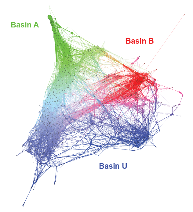
Let's see this in action. We'll start by reading in a set of three basins: $A$, $B$ and $U$.
Astates = [2031,596,1923,3223,2715]
Bstates = [1550,3168,476,1616,2590]
Ustates = list(np.loadtxt('state_U.dat',dtype=int))
We can then use the calc_committors function to calculate committors between this set of three basins. This will calculate $p_A$, $p_B$, and $p_U$ for each state, which sum to one.
basins = [Astates,Bstates,Ustates]
labels = ['pA','pB','pU']
comms = our_csn.calc_committors(basins,labels=labels)
The committors can be interpreted as follows:
i = our_csn.trim_indices[0]
print('comms['+str(i)+'] = ',comms[i])
print('\nIn other words, if you start in state {0:d}:'.format(i))
print('You will reach basin A first with probability {0:.2f}, basin B with probability {1:.2f} and basin U with probability {2:.2f}'.format(comms[i,0],comms[i,1],comms[i,2]))
comms[0] =  [0.26406217 0.29477873 0.44115911]

In other words, if you start in state 0:
You will reach basin A first with probability 0.26, basin B with probability 0.29 and basin U with probability 0.44
5) Exporting graph for visualization in Gephi
NetworkX is great for doing graph-based analyses, but not stellar at greating graph layouts for large(r) networks. However, they do have excellent built-in support for exporting graph objects in a variety of formats.
Here we'll use the .gexf format to save our network, as well as all of the attributes we've calculated, to a file that can be read into Gephi, a powerful graph visualization program. While support for Gephi has been spotty in the recent past, it is still one of the best available options for graph visualization.
Before exporting to .gexf, let's use the committors we've calculated to add colors to the nodes:
rgb = our_csn.colors_from_committors(comms)
our_csn.set_colors(rgb)
Now we have added some properties to our nodes under 'viz', which will be interpreted by Gephi:
our_csn.graph.node[0]
{'label': 0,
 'count': 482,
 'trim': 0.0,
 'eig_weights': 0.002595528367725156,
 'mult_weights': 0.0025955283677248217,
 'pA': 0.26406216543613925,
 'pB': 0.2947787254045238,
 'pU': 0.4411591091593356,
 'viz': {'color': {'r': 152, 'g': 170, 'b': 255, 'a': 0}}}
And we can use an internal networkx function to write all of this to a .gexf file:
nx.readwrite.gexf.write_gexf(our_csn.graph.to_undirected(),'test.gexf')
After opening this file in Gephi, I recommend creating a layout using the "Force Atlas 2" algorithm in the layout panel. I set the node sizes to the "eig_weights" variable, and after exporting to pdf and adding some labels, I get the following:
That's the end of our tutorial! I hope you enjoyed it and you find CSNAnalysis useful in your research. If you are having difficulties with the installation or running of the software, feel free to create an issue on the Github page.