![]()
![]()
Synchronizing Around the S Module
To "synchronize" is a lot like to "omni-triangulate" i.e. to well-order in space and/or time. "Synchronized swimming" is where they don't crash into each other, the whole point being to show off tightly coreographed dance moves.
In this Notebook we cross-check our way of deriving a tetrahedron's volume, against published edge lengths and an expected outcome. By enlisting sympy, we gain access to arbitrary precision decimals.
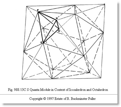
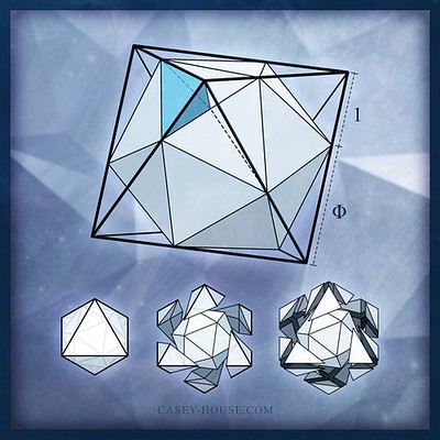
Let's start with a published page from Synergetics (R. Buckminster Fuller), showing clearly what we mean by "the S module":
Corresponding to this picture, is the corresponding plane net (note that the letters match):
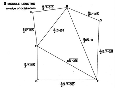
What we're going to need are the six edges of the S module tetrahedron, for one of our tetravolume computing algorithms, the ones that eat edges for input. To this end, let's gather all the distances in the above diagram.
Note that the plane net contains duplicate edges. We will make sure our labels are alphabetized internally i.e. given EG and GE, we will pick EG as the canonical representation, because E < G in the alphabet.
import pandas as pd
import numpy as np

import math
from math import sqrt as rt2

a  = 1

EF = a * rt2(7 - 3 * rt2(5))
EG = (a/2) * rt2(7 - 3 * rt2(5))
EH = (a/2) * (3 - rt2(5))
FG = (a/2) * rt2(3) * rt2(7 - 3 * rt2(5))
FH = (a/2) * (rt2(5) - 1)
GH = (a/2) * rt2(7 - 3 * rt2(5))

S_net = pd.DataFrame({'Edges'  : ['EF', 'EG', 'EH', 'FG', 'FH', 'GH'],
                      'Lengths': [EF, EG, EH, FG, FH, GH]})

S_net
| Edges | Lengths | |
|---|---|---|
| 0 | EF | 0.540182 |
| 1 | EG | 0.270091 |
| 2 | EH | 0.381966 |
| 3 | FG | 0.467811 |
| 4 | FH | 0.618034 |
| 5 | GH | 0.270091 |
Now we want a volume formula that eats edge lengths in a particular order, and returns volume.
We have at least three to choose from:
- Piero della Francesca's
- Gerald de Jong's
- Cayley-Menger Determinant
All three are described here.
We start with an apex vertex (any vertex), say E, extending to EF, EG, EH, and then we go around the opposite face in the same order i.e. FG GH FH.
Here we go then:
def CM_ivm(a, b, c, d, e, f):
    # double and 2nd power us
    A,B,C,D,E,F = [(2*x)**2 for x in (a,b,c,d,e,f)]

    # Construct a 5x5 matrix per Caley-Menger
    M = np.ones((5,5))
    M[0,0:5] = 0, 1, 1, 1, 1
    M[1,0:5] = 1, 0, A, B, C
    M[2,0:5] = 1, A, 0, D, F
    M[3,0:5] = 1, B, D, 0, E
    M[4,0:5] = 1, C, F, E, 0
    print(M) # comment out?
    return math.sqrt(np.linalg.det(M))/16  # Syn3 factored in
The reference prime vector length is set to 1 in this formula, meaning the octahedron in which the icosahedron is inscribed, and what's left with the 24 S modules subtracted, is the diameter of a unit radius IVM sphere.
CM_ivm(EF, EG, EH, FG, GH, FH)
[[0.         1.         1.         1.         1.        ]
 [1.         0.         1.16718427 0.29179607 0.58359214]
 [1.         1.16718427 0.         0.8753882  1.52786405]
 [1.         0.29179607 0.8753882  0.         0.29179607]
 [1.         0.58359214 1.52786405 0.29179607 0.        ]]
0.045084971874737007
What's our usual value for the S mod volume?
φ         = (rt2(5)+1)/2   # golden ratio
Smod      = (φ**-5) / 2    # home base Smod
Smod
0.04508497187473711
Another Synergetics motif has been the S_Factor, or S_volume / E_volume...
The 2.5 volume cuboctahedron, connecting mid-points of the containing volume 4 octahedron, transforms into an icosahedron when its 12 vertices travel from these midpoints, to new positions consistent with the 12 vertices of the faces-flush icosahedron.
This motion, akin to the Jitterbug but with edges changing length, is tantamount to multiplying the initial volume of 2.5 times the S_Factor, times the S_Factor (i.e. times the S_Factor to the 2nd power).
Emod      = (rt2(2) / 8) * (φ**-3)  # home base Emod
S_factor  = Smod / Emod  # 2*sqrt(7-3*sqrt(5))
icosa_within = 2.5 * S_factor * S_factor
icosa_within
2.9179606750063085
icosa_within + 24 * Smod
3.999999999999999
Recomputing the S Module with sympy
That's the target Octahedron volume, or close. The next step is to audit the above using sympy and its arbitrary precision numbers.
from sympy import symbols, sqrt as rt2, Matrix, ones
import sympy as sy
a = symbols('a')
EF = a * rt2(7 - 3 * rt2(5))
EG = (a/2) * rt2(7 - 3 * rt2(5))
EH = (a/2) * (3 - rt2(5))
FG = (a/2) * rt2(3) * rt2(7 - 3 * rt2(5))
FH = (a/2) * (rt2(5) - 1)
GH = (a/2) * rt2(7 - 3 * rt2(5))
EF
FH
FH.evalf(60,subs={a: 1}) # to 60 decimal places
S_net = pd.DataFrame({'Edges'  : ['EF', 'EG', 'EH', 'FG', 'FH', 'GH'],
                      'Lengths': [EF, EG, EH, FG, FH, GH],
                      'Values' : [L.evalf(60, subs={a:1})
                                  for L in [EF, EG, EH, FG, FH, GH]]})

S_net.set_index('Edges', inplace=True)
S_net
| Lengths | Values | |
|---|---|---|
| Edges | ||
| EF | a*sqrt(7 - 3*sqrt(5)) | 0.54018151347545290720308631409818785099473024... |
| EG | a*sqrt(7 - 3*sqrt(5))/2 | 0.27009075673772645360154315704909392549736512... |
| EH | a*(3 - sqrt(5))/2 | 0.38196601125010515179541316563436188227969082... |
| FG | sqrt(3)*a*sqrt(7 - 3*sqrt(5))/2 | 0.46781091332446829000553859902741320909259887... |
| FH | a*(-1 + sqrt(5))/2 | 0.61803398874989484820458683436563811772030917... |
| GH | a*sqrt(7 - 3*sqrt(5))/2 | 0.27009075673772645360154315704909392549736512... |
S_net.info()
<class 'pandas.core.frame.DataFrame'>
Index: 6 entries, EF to GH
Data columns (total 2 columns):
 #   Column   Non-Null Count  Dtype
---  ------   --------------  -----
 0   Lengths  6 non-null      object
 1   Values   6 non-null      object
dtypes: object(2)
memory usage: 144.0+ bytes
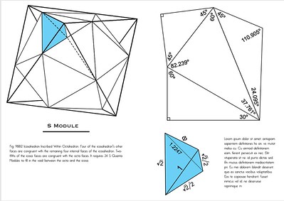
In the following cells, we compute ratios, such as EG/EH, EF/EH, FH/EH, netting $\sqrt{2}/2$, $\sqrt{2}$, and $\phi$ respectively. We're using pandas syntax to look up the numbers in the Values column, per whatever indexed rows.
If the S-modules were scaled such that EH = 1, the same ratios would obtain as in the figure below, as the other edges would likewise be scaled accordingly.
by Casey House (Syn-U)
by Casey House (Syn-U)
def L(edge):
    "lookup named edge and return the pre-computed length"
    return S_net.loc[edge].Values  # consult the DataFrame
L('EG')/L('EH') # EG/EH = rt2(2)/2
sy.N(rt2(2)/2, 60)
L('EF')/L('EH') # EF/EH = rt2(2)
sy.N(rt2(2), 60)
φ         = (rt2(5)+1)/2   # golden ratio
φ
L('FH')/L('EH') # FH/EH = φ
φ.evalf(60)
L('FG')/L('EH') # FH/EH = φ
Now it's time to recast the Cayley-Menger matrix using sympy instead of numpy. We'll be able to use arbitrary precision inputs.
def CM_ivm(a, b, c, d, e, f):
    # double and 2nd power us
    A,B,C,D,E,F = [(2*x)**2 for x in (a,b,c,d,e,f)]

    # Construct a 5x5 matrix per Caley-Menger
    M = Matrix(
        [
        [0, 1, 1, 1, 1],
        [1, 0, A, B, C],
        [1, A, 0, D, F],
        [1, B, D, 0, E],
        [1, C, F, E, 0]])
    # print(M) # comment out?
    return rt2(M.det())/16  # Syn3 factored in
args = S_net.loc[['EF', 'EG', 'EH', 'FG', 'GH', 'FH'], 'Values'] # lookup in order
args
Edges
EF    0.54018151347545290720308631409818785099473024...
EG    0.27009075673772645360154315704909392549736512...
EH    0.38196601125010515179541316563436188227969082...
FG    0.46781091332446829000553859902741320909259887...
GH    0.27009075673772645360154315704909392549736512...
FH    0.61803398874989484820458683436563811772030917...
Name: Values, dtype: object
Svol = CM_ivm(*args)  # pass to Cayley-Menger algorithm, adjusted for tetravolumes
Svol
Svol2 = (φ**-5) / 2
Svol2
We have attained our expected target volume, per the Koski Identities, for the S module.
Svol2 = Svol2.evalf(60)
Svol2
Svol
Looking good!
Evol      = (rt2(2) / 8) * (φ**-3)  # home base Emod
S_factor  = Svol / Evol  # 2*sqrt(7-3*sqrt(5))
2.5 * S_factor.evalf(60)**2
Svol
icosa_within = 2.5 * S_factor.evalf(60) * S_factor.evalf(60)
icosa_within + 24 * Svol
Yup!