2.4 Deep Taylor Decomposition Part 1.
Introduction
This section corresponds to Section 5.2 of the original paper.
I recommend reviewing Section 2.2 before reading this section.
In the previous section, we induced the LRP-$\alpha \beta$ rule through a series of constraints. Deep Taylor Decomposition is also a variant of LRP that is based upon Taylor Decomposition. In Simple Taylor Decomposition (Section 2.2), we applied Taylor Expansion to the entire network without considering the structure of DNN. However, in Deep Taylor Decomposition, we will apply Taylor Expansion in a layer-wise manner, much like how we propagated relevance layer by layer in the LRP-$\alpha \beta$ tutorial. I will show the application of Taylor Expansion to a simplified one-layer network. Deep Taylor Decomposition is simple once the one-layer version is derived, since all we have to do is to apply the one-layer version iteratively from output layer to input layer.
I will restate the three constraints below so we can refer back to it whenever necessary.
Constraint 1. $R(x_i) > 0$ should indicate positive contribution and $R(x_i) < 0$ negative contribution. If the range of $R$ is limited to nonnegative numbers, $R(x_i) = 0$ indicates no contribution and $R(x_i) > 0$ indicates positive contribution (Section 2.1).
Constraint 2. Relevance Conservation Constraint (Section 2.2):
\begin{equation} f(x) = \sum^V_{i=1} R(x_i) \end{equation}Constraint 3. Layer-wise Relevance Conservation Constraint: total relevance must be preserved throughout layers (Section 3.1).
\begin{equation} f(x) = \cdots = \sum_{d = 1}^{V(l+1)} R^{(l+1)}_d = \sum_{d = 1}^{V(l)} R^{(l)}_d = \cdots = \sum_{i = 1}^{V(1)} R^{(1)}_d \end{equation}Notations
Let us review the notations before moving onto the algorithm.
\begin{equation*} R_{i \leftarrow j}^{(l,l+1)} \end{equation*}The above notation denotes the portion of relevance distributed from neuron $j$ of layer $l+1$ to neuron $i$ of layer $l$.
\begin{equation*} R_{i}^{(l)} \end{equation*}This denotes the total relevance allocated to neuron $i$ of layer $l$. $R_{i \leftarrow j}^{(l,l+1)}$, $R_{i}^{(l)}$ and $R_{j}^{(l+1)}$ are related by the Layer-wise Relevance Conservation Constraint:
\begin{align*} \sum_i R_{i \leftarrow j}^{(l,l+1)} & = R_{j}^{(l+1)} \\ \sum_j R_{i \leftarrow j}^{(l,l+1)} & = R_{i}^{(l)} \end{align*}Application to One-layer Networks
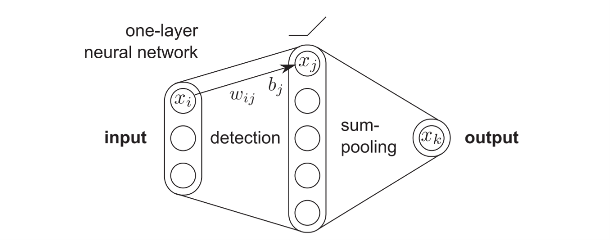
Consider a simple three-layer ReLU network. The original paper says it's an one-layer network, but I will treat it as a three-layer network throughout this tutorial for clarity and coherence of notation. Then, we can define the network as:
\begin{equation} x_j = \max \left( 0, \sum_i x_i w_{ij} + b_j \right) \end{equation}and \begin{equation} x_k = \sum_j x_j \end{equation} where $\{x_i\}$ is a $d$-dimensional input, $\{x_j\}$ is a detection layer, $x_k$ is the output and $w_{ij}$ and $b_j$ are the weight and bias parameters of the network. The mapping $\{x_i\} \rightarrow x_k$ then defines a function $f$. We now perform the Taylor Decomposition of this network. We will set an additional constraint on biases, where we force $b_j \leq 0$ for all $j$. This constraint ensures the existance of a root point $\{\tilde{x}_i\}$ of the function $f$ and therefore allows us to apply Taylor Decomposition which requires a root point.
Relevance distribution from output to detection layer
Since we must satisfy the Layer-wise Relevance Conservation Constraint, we start by equating the predicted output to the amount of total relevance that must be backpropagated, i.e., $R_{k}^{(3)} = x_k$. The relevance for the top layer can now be expressed in terms of lower-layer neurons as:
\begin{equation} R_{k}^{(3)} = \sum_j x_j \end{equation}Having established the mapping between $\{x_j\}$ and $R_{k}^{(3)}$, we would like to redistribution $R_{k}^{(3)}$ onto neurons $\{x_j\}$. Instead of using the LRP-$\alpha \beta$ rule as we did in the previous section, we apply Taylor Decomposition. Then the redistributed relevances $R_j$ can be written as:
\begin{equation} R_{j \leftarrow k}^{(2,3)} = \frac{\partial R_{k}^{(3)}}{\partial x_j} |_{\{\tilde{x}_j\}} \cdot (x_j - \tilde{x}_j) \end{equation}where $\{\tilde{x}_j\}$ is the root point, i.e., $\sum_j \tilde{x}_j = 0$. Note that since there is only one output neuron, $R_{j}^{(2)} = \sum_k R_{j \leftarrow k}^{(2,3)} = R_{j \leftarrow k}^{(2,3)}$.
Finding the root point is simple. Because $x_j = \max \left( 0, \sum_i x_i w_{ij} + b_j \right)$, $x_j$ must be nonnegative. The only point that is both a root ($\sum_j \tilde{x}_j = 0$) and nonnegative ($\forall \ j : \tilde{x}_j \geq 0$) is $\{\tilde{x}_j\} = 0$. Plugging this root into Eq. (6) and using the fact that $\partial R_{k}^{(3)} / \partial x_j = 1$, we obtain the first rule for relevance distribution:
\begin{equation} R_{j}^{(2)} = x_j \end{equation}In other words, the relevance must be redistributed on the neurons of the detection layer in the same proportion as their activation value. Trivially, we can also verify that the relevance is conserved during the redistribution process ($\sum_j R_{j}^{(2)} = \sum_j x_j = R_{k}^{(3)}$).
Relevance distribution from detection to input layer
Let us now express the relevance $R_{j}^{(2)}$ as a function of the input neurons $\{x_i\}$. Since we have $R_{j}^{(2)} = x_j$ by Eq. (7), we can write
\begin{equation} R_{j}^{(2)} = \max \left( 0, \sum_i x_i w_{ij} + b_j \right) \end{equation}This establishes a mapping between $\{x_i\}$ and $R_{j}^{(2)}$. We will again apply Taylor Decomposition to derive $R_{i}^{(1)}$ as follows
\begin{equation} R_{i \leftarrow j}^{(1,2)} = \frac{\partial R_{j}^{(2)}}{\partial x_i} |_{\{\tilde{x}_i\}^{(j)}} \cdot (x_i - \tilde{x}_i^{(j)}) \end{equation}where $\{\tilde{x}_i\}^{(j)}$ are the set of root points for which $\max \left( 0, \sum_i \tilde{x}_i^{(j)} w_{ij} + b_j \right) = x_j = 0$. By the Layer-wise Relevance Conservation Constraint
\begin{equation} R_{i}^{(1)} = \sum_j \frac{\partial R_{j}^{(2)}}{\partial x_i} |_{\{\tilde{x}_i\}^{(j)}} \cdot (x_i - \tilde{x}_i^{(j)}) \end{equation}Relevances $\{R_i\}$ can therefore be obtained by performing as many Taylor Decompositions as there are neurons in the hidden layer.
Various Propagation Rules
We will now consider various methods for choosing a root $\{\tilde{x}_i\}^{(j)}$ that takes the diversity of possible input domain $\mathcal{X} \subseteq \mathbb{R}^d$ to which the data belongs. Different choice of input domain leads to a different rule for propagating relevance from $\{R_{j}^{(2)}\}$ to $\{R_{i}^{(1)}\}$. For pooling layers (e.g., max-pooling, sum-pooling), we use the same propagation rules as those of LRP-$\alpha \beta$. As I said in the introduction, once we derive the propagation rules, we only have to apply them from the output layer to the input layer in order to achieve Deep Taylor Decomposition.
Unconstrained input space $\mathcal{X} = \mathbb{R}^d$ and the $w^2$-rule
We first consider the simplest case where any real-valued input is valid. In that case, we can always choose the root point $\{\tilde{x}_i\}^{(j)}$ that is nearest to the actual data point $\{x_i\}$ under the Euclidean norm (since we are using first-order Taylor Expansion, we must choose the closest root in order to minimize the residual error: review Section 2.2, footnote 1). We know that the root must satisfy the plane equation $\sum_i \tilde{x}_i^{(j)} w_{ij} + b_j = 0 $. Since $\mathbf{w}_j$ is the normal vector of the plane, we can derive the line of maximum descent $\{\tilde{x}_i\}^{(j)} = \{x_i\} + t \cdot \mathbf{w}_j$ where $t \in \mathbb{R}$. Because the line intersects perpendicularly with the plane, the intersection of those two subspaces gives us the nearest root point. With that root point, we can express $R_{i \leftarrow j}^{(1,2)}$ in terms of $w_{ij}$ and $R_{j}^{(2)}$. Calculation process is given below.
First we derive $\tilde{x}_i^{(j)}$ in terms of $x_i$, $w_{ij}$ and $b_j$. \begin{align} \sum_i \tilde{x}_i^{(j)} w_{ij} + b_j = 0 \\ \sum_i (x_i + t w_{ij}) w_{ij} + b_j = 0 \\ \sum_i (x_i w_{ij} + t w_{ij}^2) + b_j = 0 \\ \sum_i x_i w_{ij} + t \sum_i w_{ij}^2 + b_j = 0 \\ t = \frac{-1}{\sum_i w_{ij}^2} \left( \sum_i x_i w_{ij} + b_j \right) \\ \tilde{x}_{i}^{(j)} = x_i - \frac{w_{ij}}{\sum_i w_{ij}^2} \left( \sum_i x_i w_{ij} + b_j \right) \end{align}
Now we calculate the partial derivative of $R_{j}^{(2)}$ with respect to $x_i$. \begin{align} R_{j}^{(2)} = \max \left( 0, \sum_i x_i w_{ij} + b_j \right) \\ \frac{\partial R_{j}^{(2)}}{\partial x_i} = w_{ij} \end{align}
Now we are ready to calculate $R_{i \leftarrow j}^{(1,2)}$. \begin{align} R_{i \leftarrow j}^{(1,2)} & = \frac{\partial R_{j}^{(2)}}{\partial x_i} |_{\{\tilde{x}_i\}^{(j)}} \cdot (x_i - \tilde{x}_i^{(j)}) \\ & = \frac{w_{ij}^2}{\sum_{i} w_{ij}^2} \left( \sum_i x_i w_{ij} + b_j \right) \\ & = \frac{w_{ij}^2}{\sum_{i} w_{ij}^2} R_{j}^{(2)} \end{align}
Total relevance can be calculated by the Layer-wise Relevance Conservation Constraint. \begin{equation} R_{i}^{(1)} = \sum_j \frac{w_{ij}^2}{\sum_{i'} w_{i'j}^2} R_{j}^{(2)} \end{equation}
We call this propagation method the $w^2$-rule.
Constrained input space $\mathcal{X = \mathbb{R}_{+}^{d}}$ and the $z^+$-rule
We now consider the case $\mathcal{X = \mathbb{R}_{+}^{d}}$ where the input values are constrained to be positive, e.g., the activations of ReLU neurons. In that case, we restrict the search domain to the segment $(\{x_i 1_{w_{ij} < 0}\}, \{x_i\}) \subset \mathbb{R}_+^d$ that is guaranteed to have at least one root $\{\tilde{x}_i\}^{(j)} = \{x_i 1_{w_{ij} < 0}\}$ (you can verify this fact by checking that $\sum_i (x_i 1_{w_{ij} < 0}) w_{ij} \leq 0$ and therefore the ReLU activation value is $0$.)
We can derive the propagation rule through the following series of calculations:
Since the search domain is restricted to $(\{x_i 1_{w_{ij} < 0}\}, \{x_i\})$, we need a different expression for $\tilde{x}_i^{(j)}$:
\begin{equation} \tilde{x}_i^{(j)} = \left( 1 + t \frac{w_{ij}^+}{w_{ij}} \right) x_i = x_i + t x_i \frac{w_{ij}^+}{w_{ij}} \end{equation}where $t \in (-1,0)$ and $w_{ij}^+$ denotes the positive part of $w_{ij}$.
We can now express $\tilde{x}_i^{(j)}$ in terms of $x_i$, $w_{ij}$ and $b_j$. \begin{align} \sum_i \tilde{x}_i^{(j)} w_{ij} + b_j = 0 \\ \sum_i \left( x_i + t x_i \frac{w_{ij}^+}{w_{ij}} \right) w_{ij} + b_j = 0 \\ \sum_i (x_i w_{ij} + t x_i w_{ij}^+) + b_j = 0 \\ \sum_i x_i w_{ij} + t \sum_i x_i w_{ij}^+ + b_j = 0 \\ t = \frac{-1}{\sum_i x_i w_{ij}^+} \left( \sum_i x_i w_{ij} + b_j \right) \\ \tilde{x}_{i}^{(j)} = x_i - \frac{x_i w_{ij}^+}{w_{ij} \sum_i x_i w_{ij}^+} \left( \sum_i x_i w_{ij} + b_j \right) \end{align}
We reuse the results of Eq. (18) for the partial derivative calculation. Now we are ready to calculate $R_{i \leftarrow j}^{(1,2)}$.
\begin{align} R_{i \leftarrow j}^{(1,2)} & = \frac{\partial R_{j}^{(2)}}{\partial x_i} |_{\{\tilde{x}_i\}^{(j)}} \cdot (x_i - \tilde{x}_i^{(j)}) \\ & = w_{ij} \cdot \frac{x_i w_{ij}^+}{w_{ij} \sum_i x_i w_{ij}^+} \left( \sum_i x_i w_{ij} + b_j \right) \\ & = \frac{x_i w_{ij}^+}{\sum_i x_i w_{ij}^+} R_{j}^{(2)} \\ & = \frac{z_{ij}^+}{\sum_i z_{ij}^+} R_{j}^{(2)} \end{align}where $z_{ij}^+ = x_i w_{ij}^+$.
Total relevance can be calculated by the Layer-wise Relevance Conservation Constraint. \begin{equation} R_{i}^{(1)} = \sum_j \frac{z_{ij}^+}{\sum_{i'} z_{i'j}^+} R_{j}^{(2)} \end{equation}
We call this propagation method the $z^+$-rule. Note that this method is exactly the LRP-$\alpha_1 \beta_0$ rule we derived in Section 3.1.
$z^+$-rule implementation for dense and convolution layers
def backprop_dense(self, activation, kernel, relevance):
    W_p = tf.maximum(0., kernel)
    z = tf.matmul(activation, W_p) + 1e-10
    s = relevance / z
    c = tf.matmul(s, tf.transpose(W_p))
    return activation * c

def backprop_conv(self, activation, kernel, relevance, strides, padding='SAME'):
    W_p = tf.maximum(0., kernel)
    z = nn_ops.conv2d(activation, W_p, strides, padding) + 1e-10
    s = relevance / z
    c = nn_ops.conv2d_backprop_input(tf.shape(activation), W_p, s, strides, padding)
    return activation * c
Constrained input space $\mathcal{B} = \{\{x_i\}: \forall_{i=1}^d l_i \geq x_i \geq h_i\}$ and the $z^{\mathcal{B}}$-rule
For image classification tasks, pixel values are typically bounded above and below. That is, they exist within a box $\mathcal{B} = \{\{x_i\}: \forall_{i=1}^d l_i \geq x_i \geq h_i\}$ where $l_i \leq 0$ and $h_i \geq 0$ are the smallest and largest allowed pixel values for each dimension. In that case, we can restrict the search domain to the segment $(\{l_i 1_{w_{ij} > 0} + h_i 1_{w_{ij} < 0}\}, \{x_i\}) \subset \mathcal{B}$ that is also guaranteed to have at least one root $\{l_i 1_{w_{ij} > 0} + h_i 1_{w_{ij} < 0}\}$ ($\sum_i (l_i 1_{w_{ij} > 0} + h_i 1_{w_{ij} < 0}) w_{ij} \leq 0$ and therefore the ReLU activation value is $0$).
We can derive the propagation rule through the following series of calculations:
Since the search domain is restricted to $(\{l_i 1_{w_{ij} > 0} + h_i 1_{w_{ij} < 0}\})$, we need a different expression for $\tilde{x}_i^{(j)}$:
\begin{equation} \tilde{x}_i^{(j)} = x_i + t \left( x_i - \frac{w_{ij}^+}{w_{ij}} l_i - \frac{w_{ij}^-}{w_{ij}} h_i \right) \end{equation}where $t \in (-1,0)$ and $w_{ij}^+$ and $w_{ij}^-$ denote the positive and negative parts of $w_{ij}$.
We can now express $\tilde{x}_i^{(j)}$ in terms of $x_i$, $w_{ij}$ and $b_j$. \begin{align} \sum_i \tilde{x}_i^{(j)} w_{ij} + b_j = 0 \\ \sum_i \left( x_i + t \left( x_i - \frac{w_{ij}^+}{w_{ij}} l_i - \frac{w_{ij}^-}{w_{ij}} h_i \right) \right) w_{ij} + b_j = 0 \\ \sum_i (x_i w_{ij} + t (x_i w_{ij} - l_i w_{ij}^+ - h_i w_{ij}^-)) + b_j = 0 \\ \sum_i x_i w_{ij} + t \sum_i (x_i w_{ij} - l_i w_{ij}^+ - h_i w_{ij}^-) + b_j = 0 \\ t = \frac{-1}{\sum_i (x_i w_{ij} - l_i w_{ij}^+ - h_i w_{ij}^-)} \left( \sum_i x_i w_{ij} + b_j \right) \\ \tilde{x}_{i}^{(j)} = x_i - \frac{x_i w_{ij} - l_i w_{ij}^+ - h_i w_{ij}^-}{w_{ij} \sum_i (x_i w_{ij} - l_i w_{ij}^+ - h_i w_{ij}^-)} \left( \sum_i x_i w_{ij} + b_j \right) \end{align}
We reuse the results of Eq. (18) for the partial derivative calculation. Now we are ready to calculate $R_{i \leftarrow j}^{(1,2)}$.
\begin{align} R_{i \leftarrow j}^{(1,2)} & = \frac{\partial R_{j}^{(2)}}{\partial x_i} |_{\{\tilde{x}_i\}^{(j)}} \cdot (x_i - \tilde{x}_i^{(j)}) \\ & = w_{ij} \cdot \frac{x_i w_{ij} - l_i w_{ij}^+ - h_i w_{ij}^-}{w_{ij} \sum_i (x_i w_{ij} - l_i w_{ij}^+ - h_i w_{ij}^-)} \left( \sum_i x_i w_{ij} + b_j \right) \\ & = \frac{x_i w_{ij} - l_i w_{ij}^+ - h_i w_{ij}^-}{\sum_i x_i w_{ij} - l_i w_{ij}^+ - h_i w_{ij}^-} R_{j}^{(2)} \\ & = \frac{z_{ij} - l_i w_{ij}^+ - h_i w_{ij}^-}{\sum_i z_{ij} - l_i w_{ij}^+ - h_i w_{ij}^-} R_{j}^{(2)} \end{align}where $z_{ij} = x_i w_{ij}$.
Total relevance can be calculated by the Layer-wise Relevance Conservation Constraint.
\begin{equation} R_{i}^{(1)} = \sum_j \frac{z_{ij} - l_i w_{ij}^+ - h_i w_{ij}^-}{\sum_{i'} z_{i'j} - l_i w_{i'j}^+ - h_i w_{i'j}^-} R_{j}^{(2)} \end{equation}We call this propagation method the $z^{\mathcal{B}}$-rule.
$z^{\mathcal{B}}$-rule implementation for dense and convolution layers
def backprop_dense_input(self, X, kernel, relevance, lowest=0., highest=1.):
    W_p = tf.maximum(0., kernel)
    W_n = tf.minimum(0., kernel)

    L = tf.ones_like(X, tf.float32) * lowest
    H = tf.ones_like(X, tf.float32) * highest

    z_o = tf.matmul(X, kernel)
    z_p = tf.matmul(L, W_p)
    z_n = tf.matmul(H, W_n)

    z = z_o - z_p - z_n + 1e-10
    s = relevance / z

    c_o = tf.matmul(s, tf.transpose(kernel))
    c_p = tf.matmul(s, tf.transpose(W_p))
    c_n = tf.matmul(s, tf.transpose(W_n))

    return X * c_o - L * c_p - H * c_n

def backprop_conv_input(self, X, kernel, relevance, strides, padding='SAME', lowest=0., highest=1.):
    W_p = tf.maximum(0., kernel)
    W_n = tf.minimum(0., kernel)

    L = tf.ones_like(X, tf.float32) * lowest
    H = tf.ones_like(X, tf.float32) * highest

    z_o = nn_ops.conv2d(X, kernel, strides, padding)
    z_p = nn_ops.conv2d(L, W_p, strides, padding)
    z_n = nn_ops.conv2d(H, W_n, strides, padding)

    z = z_o - z_p - z_n + 1e-10
    s = relevance / z

    c_o = nn_ops.conv2d_backprop_input(tf.shape(X), kernel, s, strides, padding)
    c_p = nn_ops.conv2d_backprop_input(tf.shape(X), W_p, s, strides, padding)
    c_n = nn_ops.conv2d_backprop_input(tf.shape(X), W_n, s, strides, padding)

    return X * c_o - L * c_p - H * c_n