How Autoencoders work - Understangin the math and implementation
이 커널은 Shivam Bansal님의 오토인코더 예시을 번역한 커널입니다.
original kernel : https://www.kaggle.com/shivamb/how-autoencoders-work-intro-and-usecases
Thanks to @ShivamBansal for awesome kernel about Autoencoder.
Contents
- Introduction
- 1.1 What are Autoencoders ?
- 1.2 How Autoencoders Work ?
- Implementation and UseCases
- 2.1 UseCase 1: Image Reconstruction
- 2.2 UseCase 2: Noise Removal
- 2.3 UseCase 3: Sequence to Sequence Prediction
더 많은 좋은 자료를 만들려고 노력하고 있습니다.
- 블로그 : 안수빈의 블로그
- 페이스북 : 어썸너드 수비니움
- 유튜브 : 수비니움의 코딩일지
1. Introduction
1.1 오토인코더란 무엇인가?
오토인코더는 입력을 그대로 똑같이 출력을 만드는 특별한 유형의 신경망입니다. 오토인코더는 비지도 학습으로 입력 데이터에 대한 low-level의 성질을 학습하기 위해 사용합니다. 이런 low-level 성질은 실제 데이터로 재구성하는데 도움을 줍니다.
오토인코더는 네트워크가 입력을 예측하도록 요구하는 회귀작업이라고 볼 수 있습니다. 이 네트워크는 중간에 병목 현상이 있고, 이런 병목은 후에 디코더로 원본 데이터로 다시 변환하기 위해 필요한 입력 데이터를 효과적인 표현으로 압축해주는 효과를 가집니다.
이런 오토 인코더는 3가지 구성 요소가 있습니다.
Encoding Architecture : 인코더 구조는 일련의 레이어로 구성되고, 이를 이용해 노드를 감소시킵니다. 그리고 잠재 공간 표현의 크기를 매우 줄여줍니다.
Latent View Representation : 잠복 공간은 줄어든 입력 정보가 보존되는 가장 낮은 레벨 공간을 나타냅니다.
Decoding Architecture : 인코딩 구조와 대칭되는 거울상이지만, 모든 레이어의 노드 수가 증가하고 궁극적으로 거의 유사한 입력을 출력합니다.
Latent View를 저는 다른 문서에서 많이 사용하는 latent space라 생각하여 잠재공간 로 번역했습니다.

매우 섬세하게 조정된 오토인코딩 모델은 첫 번째 레이어에서 전달된 동일한 입력을 재구성 할 수 있어야합니다. 이 커널(필사)에서는 오토인코더와 그 구현 방법을 설명합니다.
오토인코더는 이미지 데이터에 많이 사용되고, 다음과 같은 사례에서 사용할 수 있습니다.
- 차원 축소
- 이미지 압축
- 이미지 노이즈 제거
- 이미지 생성
- 특성 추출
1.2 How Autoencoder work
오토인코더의 수학적 배경에 대해 먼저 알아보겠습니다. 가장 기본이 되는 아이디어는 '고차원 데이터에서 저차원 표현을 학습하는 것' 입니다.
예제를 통해 알아보도록 하겠습니다. 데이터를 표현할 공간과, 두 개의 변수(x1, x2)로 나타낼 수 있는 데이터를 생각해봅시다. 데이터 매니폴드는 실제 데이터가 존재하는 데이터 표현 공간 내부의 공간입니다.
from plotly.offline import init_notebook_mode, iplot
import plotly.graph_objs as go
import numpy as np
init_notebook_mode(connected=True)

## generate random data
N = 50
random_x = np.linspace(2, 10, N)
random_y1 = np.linspace(2, 10, N)
random_y2 = np.linspace(2, 10, N)

trace1 = go.Scatter(x = random_x, y = random_y1, mode="markers", name="Actual Data")
trace2 = go.Scatter(x = random_x, y = random_y2, mode="lines", name="Model")
layout = go.Layout(title="2D Data Repersentation Space", xaxis=dict(title="x2", range=(0,12)),
                   yaxis=dict(title="x1", range=(0,12)), height=400,
                   annotations=[dict(x=5, y=5, xref='x', yref='y', text='This 1D line is the Data Manifold (where data resides)',
                   showarrow=True, align='center', arrowhead=2, arrowsize=1, arrowwidth=2, arrowcolor='#636363',
                   ax=-120, ay=-30, bordercolor='#c7c7c7', borderwidth=2, borderpad=4, bgcolor='orange', opacity=0.8)])
figure = go.Figure(data = [trace1], layout = layout)
iplot(figure)
이 데이터를 표현하기 위해서는, 2개의 차원을 사용합니다. (X축과 Y축) 하지만 다음과 같은 정보가 있다면, 이 데이터를 하나의 차원, 1D로 축소할 수 있습니다.
- 기준점 : A
- 수평선과의 각도 : L
위에 정보만 가지고 있다면 직선 위의 점 B는 거리 D로 표현가능합니다.
random_y3 = [2 for i in range(100)]
random_y4 = random_y2 + 1
trace4 = go.Scatter(x = random_x[4:24], y = random_y4[4:300], mode="lines")
trace3 = go.Scatter(x = random_x, y = random_y3, mode="lines")
trace1 = go.Scatter(x = random_x, y = random_y1, mode="markers")
trace2 = go.Scatter(x = random_x, y = random_y2, mode="lines")
layout = go.Layout(xaxis=dict(title="x1", range=(0,12)), yaxis=dict(title="x2", range=(0,12)), height=400,
                   annotations=[dict(x=2, y=2, xref='x', yref='y', text='A', showarrow=True, align='center', arrowhead=2, arrowsize=1, arrowwidth=2,
                                     arrowcolor='#636363', ax=20, ay=-30, bordercolor='#c7c7c7', borderwidth=2, borderpad=4, bgcolor='orange', opacity=0.8),
                                dict(x=6, y=6, xref='x', yref='y', text='B', showarrow=True, align='center', arrowhead=2, arrowsize=1, arrowwidth=2, arrowcolor='#636363',
                                     ax=20, ay=-30, bordercolor='#c7c7c7', borderwidth=2, borderpad=4, bgcolor='yellow', opacity=0.8), dict(
                                     x=4, y=5, xref='x', yref='y',text='d', ay=-40),
                                dict(x=2, y=2, xref='x', yref='y', text='angle L', ax=80, ay=-10)], title="2D Data Repersentation Space", showlegend=False)
data = [trace1, trace2, trace3, trace4]
figure = go.Figure(data = data, layout = layout)
iplot(figure)


#################

random_y3 = [2 for i in range(100)]
random_y4 = random_y2 + 1
trace4 = go.Scatter(x = random_x[4:24], y = random_y4[4:300], mode="lines")
trace3 = go.Scatter(x = random_x, y = random_y3, mode="lines")
trace1 = go.Scatter(x = random_x, y = random_y1, mode="markers")
trace2 = go.Scatter(x = random_x, y = random_y2, mode="lines")
layout = go.Layout(xaxis=dict(title="u1", range=(1.5,12)), yaxis=dict(title="u2", range=(1.5,12)), height=400,
                   annotations=[dict(x=2, y=2, xref='x', yref='y', text='A', showarrow=True, align='center', arrowhead=2, arrowsize=1, arrowwidth=2,
                                     arrowcolor='#636363', ax=20, ay=-30, bordercolor='#c7c7c7', borderwidth=2, borderpad=4, bgcolor='orange', opacity=0.8),
                                dict(x=6, y=6, xref='x', yref='y', text='B', showarrow=True, align='center', arrowhead=2, arrowsize=1, arrowwidth=2, arrowcolor='#636363',
                                     ax=20, ay=-30, bordercolor='#c7c7c7', borderwidth=2, borderpad=4, bgcolor='yellow', opacity=0.8), dict(
                                     x=4, y=5, xref='x', yref='y',text='d', ay=-40),
                                dict(x=2, y=2, xref='x', yref='y', text='angle L', ax=80, ay=-10)], title="Latent Distance View Space", showlegend=False)
data = [trace1, trace2, trace3, trace4]
figure = go.Figure(data = data, layout = layout)
iplot(figure)
하지만 여기서 핵심 질문은 '어떤 논리나 규칙에 의해 B가 A와 L을 통해 표현될 수 있는가' 입니다. 또 다른 말로 B, A, L간의 방정식이 어떻게 되는지를 알아야합니다.
고정된 방정식이 없어도, 비지도 학습에 의해 가능한 최상의 방정식을 구할 수 있습니다. 간단히 말해 학습 과정은 A와 L의 형태로 B를 변환하는 규칙/방정식으로 정의 할 수 있습니다. 오토인코딩 관점에서 이 과정을 이해해봅시다.
hidden layer가 없는 오토인코더를 가정해봅시다. x1, x2는 낮은 표현 d로 바뀌고, 이 d는 후에 다시 x1, x2로 투영됩니다.(변환됩니다.)

Step1 : 잠재 공간에 포인트 표현하기
A와 B를 좌표로 나타낸다면 다음과 같이 할 수 있습니다.
- Point A : (X1A,X2A)
- Point B : (X1B,X2B)
이제 이를 잠재 공간에서는 다음과 같이 표현할 수 있습니다.
- A : (X1A,X2A)→(0,0)
- B : (X1B,X2B)→(u1B,u2B)
(u1B,u2B)는 다음과 같이 기준점과의 거리로 표현할 수 있습니다.
u1B=X1B−X1A u2B=X2B−X2A
Step 2 : 거리 d와 각도 L로 포인트 표현하기
이제 u1B,u2B를 거리 d와 각도 L로 표현할 수 있습니다. 각도 L만큼 기존 축으로 회전한다면 L은 0이 될 것입니다. i.e
(d,L)→(d,0) (after rotation)
이제 이 데이터가 출력이 되고, 낮은 차원에서 표현한 입력 데이터입니다.
모든 계층의 가중치와 편향이 있는 신경망의 기본 방정식을 생각하면 다음과 같은 과정이 인코딩이라고 생각할 수 있습니다.
= ((d,0)=W⋅(u1B,u2B)
==> (encoding)
W는 hidden layer의 가중치 행렬입니다. 이후 디코딩 과정은 인코딩 과정을 반대로 생각하면 됩니다.
=> (u1B,u2B)=Inverse(W)⋅(d,0)
==> (decoding)
Different Rules for Different data
모든 유형의 데이터가 똑같은 규칙이 적용되는 것은 아닙니다. 예시로 앞에 데이터에서는 1차원 선형 데이터 매니폴드에 투영하면서 각도 L을 없앴습니다. 하지만 정확하게 투영 불가능한 데이터에 대해서는 어떨까요?
예시로 다음 데이터를 살펴봅시다.
import matplotlib.pyplot as plt
import numpy as np
fs = 100 # sample rate
f = 2 # the frequency of the signal
x = np.arange(fs) # the points on the x axis for plotting
y = [ np.sin(2*np.pi*f * (i/fs)) for i in x]

% matplotlib inline
plt.figure(figsize=(15,4))
plt.stem(x,y, 'r', );
plt.plot(x,y);

이런 유형의 데이터에서 문제점은 투영을 함과 동시에 데이터에 대한 손실을 복구할 수 없다는 것입니다. 아무리 많은 이동과 회전으로도 원본 데이터는 복구할 수 없습니다.
그렇다면 신경망은 이 문제를 어떻게 해결할까요? deep neural network는 선형 데이터를 만들기 위해 공간을 구부릴 수 있습니다. 그렇기에 오토인코더는 이런 hidden layer의 기능을 활용하여 저차원 표현을 학습할 수 있습니다.

이제 케라스를 이용하여 이미지에 오토인코더를 적용해봅시다.
## load the libraries
from keras.layers import Dense, Input, Conv2D, LSTM, MaxPool2D, UpSampling2D
from sklearn.model_selection import train_test_split
from keras.callbacks import EarlyStopping
from keras.utils import to_categorical
from numpy import argmax, array_equal
import matplotlib.pyplot as plt
from keras.models import Model
from imgaug import augmenters
from random import randint
import pandas as pd
import numpy as np
Using TensorFlow backend.
2. Dataset Prepration
데이터셋을 불러오고, 예측값과 타겟을 분리하며, 입력 데이터를 정규화합니다.
### read dataset
train = pd.read_csv("../input/fashion-mnist_train.csv")
train_x = train[list(train.columns)[1:]].values
train_y = train['label'].values

## normalize and reshape the predictors
train_x = train_x / 255

## create train and validation datasets
train_x, val_x, train_y, val_y = train_test_split(train_x, train_y, test_size=0.2)

## reshape the inputs
train_x = train_x.reshape(-1, 784)
val_x = val_x.reshape(-1, 784)
3. Create Autoencoder architecture
이제 오토인코더 구조를 만들어봅시다. 인코딩 부분은 3개의 레이어로 구성됩니다. (2000, 1200, 500 노드로 구성된) 인코딩 구조는 잠재 공간에 10개의 노드로 연결되고, 이 10개는 다시 각각 500, 1200, 2000개의 노드로 구성된 3개의 디코딩 구조로 연결됩니다. 그리고 마지막에 처음 인풋과 같은 노드의 수로 맞춰줍니다.
## input layer
input_layer = Input(shape=(784,))

## encoding architecture
encode_layer1 = Dense(1500, activation='relu')(input_layer)
encode_layer2 = Dense(1000, activation='relu')(encode_layer1)
encode_layer3 = Dense(500, activation='relu')(encode_layer2)

## latent view
latent_view   = Dense(10, activation='sigmoid')(encode_layer3)

## decoding architecture
decode_layer1 = Dense(500, activation='relu')(latent_view)
decode_layer2 = Dense(1000, activation='relu')(decode_layer1)
decode_layer3 = Dense(1500, activation='relu')(decode_layer2)

## output layer
output_layer  = Dense(784)(decode_layer3)

model = Model(input_layer, output_layer)
이제 모델을 확인해봅시다.
model.summary()
_________________________________________________________________
Layer (type)                 Output Shape              Param #
=================================================================
input_1 (InputLayer)         (None, 784)               0
_________________________________________________________________
dense_1 (Dense)              (None, 1500)              1177500
_________________________________________________________________
dense_2 (Dense)              (None, 1000)              1501000
_________________________________________________________________
dense_3 (Dense)              (None, 500)               500500
_________________________________________________________________
dense_4 (Dense)              (None, 10)                5010
_________________________________________________________________
dense_5 (Dense)              (None, 500)               5500
_________________________________________________________________
dense_6 (Dense)              (None, 1000)              501000
_________________________________________________________________
dense_7 (Dense)              (None, 1500)              1501500
_________________________________________________________________
dense_8 (Dense)              (None, 784)               1176784
=================================================================
Total params: 6,368,794
Trainable params: 6,368,794
Non-trainable params: 0
_________________________________________________________________
조기 학습 종료를 이용하여 훈련을 해보겠습니다. (early stopping callback)
model.compile(optimizer='adam', loss='mse')
early_stopping = EarlyStopping(monitor='val_loss', min_delta=0, patience=10, verbose=1, mode='auto')
model.fit(train_x, train_x, epochs=20, batch_size=2048, validation_data=(val_x, val_x), callbacks=[early_stopping])
Train on 48000 samples, validate on 12000 samples
Epoch 1/20
48000/48000 [==============================] - 4s 89us/step - loss: 0.0973 - val_loss: 0.0696
Epoch 2/20
48000/48000 [==============================] - 1s 25us/step - loss: 0.0648 - val_loss: 0.0566
Epoch 3/20
48000/48000 [==============================] - 1s 26us/step - loss: 0.0504 - val_loss: 0.0442
Epoch 4/20
48000/48000 [==============================] - 1s 26us/step - loss: 0.0407 - val_loss: 0.0382
Epoch 5/20
48000/48000 [==============================] - 1s 26us/step - loss: 0.0370 - val_loss: 0.0375
Epoch 6/20
48000/48000 [==============================] - 1s 25us/step - loss: 0.0351 - val_loss: 0.0329
Epoch 7/20
48000/48000 [==============================] - 1s 26us/step - loss: 0.0315 - val_loss: 0.0303
Epoch 8/20
48000/48000 [==============================] - 1s 26us/step - loss: 0.0294 - val_loss: 0.0278
Epoch 9/20
48000/48000 [==============================] - 1s 26us/step - loss: 0.0268 - val_loss: 0.0261
Epoch 10/20
48000/48000 [==============================] - 1s 27us/step - loss: 0.0252 - val_loss: 0.0245
Epoch 11/20
48000/48000 [==============================] - 1s 25us/step - loss: 0.0239 - val_loss: 0.0238
Epoch 12/20
48000/48000 [==============================] - 1s 25us/step - loss: 0.0235 - val_loss: 0.0229
Epoch 13/20
48000/48000 [==============================] - 1s 24us/step - loss: 0.0225 - val_loss: 0.0225
Epoch 14/20
48000/48000 [==============================] - 1s 25us/step - loss: 0.0218 - val_loss: 0.0215
Epoch 15/20
48000/48000 [==============================] - 1s 24us/step - loss: 0.0209 - val_loss: 0.0209
Epoch 16/20
48000/48000 [==============================] - 1s 25us/step - loss: 0.0207 - val_loss: 0.0204
Epoch 17/20
48000/48000 [==============================] - 1s 24us/step - loss: 0.0202 - val_loss: 0.0204
Epoch 18/20
48000/48000 [==============================] - 1s 24us/step - loss: 0.0198 - val_loss: 0.0200
Epoch 19/20
48000/48000 [==============================] - 1s 25us/step - loss: 0.0192 - val_loss: 0.0192
Epoch 20/20
48000/48000 [==============================] - 1s 25us/step - loss: 0.0189 - val_loss: 0.0190
<keras.callbacks.History at 0x7f12eeea5eb8>
검증 데이터에 예측을 생성합니다.
preds = model.predict(val_x)
원본 이미지와 예측 이미지를 그려봅시다.
Inputs : Actual Images
from PIL import Image
f, ax = plt.subplots(1,5)
f.set_size_inches(80, 40)
for i in range(5):
    ax[i].imshow(val_x[i].reshape(28, 28))
plt.show()

Predicted : Autoencoder Output
f, ax = plt.subplots(1,5)
f.set_size_inches(80, 40)
for i in range(5):
    ax[i].imshow(preds[i].reshape(28, 28))
plt.show()

20 epochs 만으로 입력 이미지를 다시 잘 구성하는 것을 확인할 수 있었습니다. 이제 오토인코더로 노이즈를 없애는 예시를 살펴봅시다.
2.2 UseCase 2 - Image Denoising
오토인코딩은 매우 유용합니다. 이제 다른 예시를 살펴보겠습니다.
많은 경우에 입력 이미지는 노이즈를 가지고 있습니다. 오토인코더는 이를 제거할 수 있습니다. 우선 train_x와 val_x 데이터를 이미지 픽셀과 함께 준비해봅시다.
## recreate the train_x array and val_x array
train_x = train[list(train.columns)[1:]].values
train_x, val_x = train_test_split(train_x, test_size=0.2)

## normalize and reshape
train_x = train_x/255.
val_x = val_x/255.
이번 오토인코더 네트워크에는 convolutional layer을 추가합니다. 왜냐하면 convolutional networks는 이미지 입력에 대해 매우 잘 작동하기 때문입니다. 입력 데이터를 convolutional network에 넣기 위해서는 28 * 28 matrix로 reshape해야합니다.
train_x = train_x.reshape(-1, 28, 28, 1)
val_x = val_x.reshape(-1, 28, 28, 1)
Noisy Images
우리는 의도적으로 이미지에 노이즈를 추가할 수 있습니다. 이미지를 보완하는 imaug 패키지를 이용하여, 반대로 이미지에 노이즈를 만들 수 있습니다. 노이즈에는 다음과 같은 것이 있습니다.
- Salt and Pepper Noise
- Gaussian Noise
- Periodic Noise
- Speckle Noise
여기서는 impulse noise라고 불리는 Salt and Pepper Noise를 사용했습니다. 이 노이즈는 선명하고 갑작스러운 노이즈를 만듭니다. 희소하게 검정/흰 픽셀을 만듭니다.
원본 커널에서 노이즈에 대해 수정해주신 @ColinMorris에게 다시 감사함을 전합니다.
Thanks to @ColinMorris for suggesting the correction in salt and pepper noise.
# Lets add sample noise - Salt and Pepper
noise = augmenters.SaltAndPepper(0.1)
seq_object = augmenters.Sequential([noise])

train_x_n = seq_object.augment_images(train_x * 255) / 255
val_x_n = seq_object.augment_images(val_x * 255) / 255
- Before adding noise
f, ax = plt.subplots(1,5)
f.set_size_inches(80, 40)
for i in range(5,10):
    ax[i-5].imshow(train_x[i].reshape(28, 28))
plt.show()

- After adding noise
f, ax = plt.subplots(1,5)
f.set_size_inches(80, 40)
for i in range(5,10):
    ax[i-5].imshow(train_x_n[i].reshape(28, 28))
plt.show()

이제 오토인코더를 위한 모델을 만들어봅시다. 어떤 종류의 네트워크가 필요한지 알아봅시다.
Encoding Architecture
인코딩 구조는 3개의 Convolutional Layer과 3개의 Max Pooling 레이어를 하나하나 쌓아 구성됩니다.
Relu를 활성화함수로 사용하고, same 매개변수로 이미지 크기를 패딩을 통해 유지합니다.
Max pooling layer의 역할은 이미지 차원을 다운샘플링하기 위해 사용됩니다. 이 레이어는 초기 표현의 겹치지 않는 부분 영역에 최대 필터를 적용합니다.
Decoding Architecture
디코딩 구조에서도 거의 유사하게 3개의 Convolutional Layer를 사용합니다. 하지만 Max Pooling layer 3개 대신에 unsampling layer 3개를 사용합니다. 활성화함수와 패딩은 인코딩과 동일합니다.
Unsampling layer의 역할은 입력 벡터를 더 높은 차원으로 업샘플링하기 위해 사용합니다. Max pooling 연산은 비가역이지만, 각 풀링 영역 내에 최대 값의 위치를 기록함으로써 근사 역을 구할 수있습니다. Umsampling 레이어는 이 속성을 사용하여 낮은 차원의 특징 공간에서 재구성합니다.
# input layer
input_layer = Input(shape=(28, 28, 1))

# encoding architecture
encoded_layer1 = Conv2D(64, (3, 3), activation='relu', padding='same')(input_layer)
encoded_layer1 = MaxPool2D( (2, 2), padding='same')(encoded_layer1)
encoded_layer2 = Conv2D(32, (3, 3), activation='relu', padding='same')(encoded_layer1)
encoded_layer2 = MaxPool2D( (2, 2), padding='same')(encoded_layer2)
encoded_layer3 = Conv2D(16, (3, 3), activation='relu', padding='same')(encoded_layer2)
latent_view    = MaxPool2D( (2, 2), padding='same')(encoded_layer3)

# decoding architecture
decoded_layer1 = Conv2D(16, (3, 3), activation='relu', padding='same')(latent_view)
decoded_layer1 = UpSampling2D((2, 2))(decoded_layer1)
decoded_layer2 = Conv2D(32, (3, 3), activation='relu', padding='same')(decoded_layer1)
decoded_layer2 = UpSampling2D((2, 2))(decoded_layer2)
decoded_layer3 = Conv2D(64, (3, 3), activation='relu')(decoded_layer2)
decoded_layer3 = UpSampling2D((2, 2))(decoded_layer3)
output_layer   = Conv2D(1, (3, 3), padding='same')(decoded_layer3)

# compile the model
model_2 = Model(input_layer, output_layer)
model_2.compile(optimizer='adam', loss='mse')
모델 정보는 다음과 같습니다.
model_2.summary()
_________________________________________________________________
Layer (type)                 Output Shape              Param #
=================================================================
input_2 (InputLayer)         (None, 28, 28, 1)         0
_________________________________________________________________
conv2d_1 (Conv2D)            (None, 28, 28, 64)        640
_________________________________________________________________
max_pooling2d_1 (MaxPooling2 (None, 14, 14, 64)        0
_________________________________________________________________
conv2d_2 (Conv2D)            (None, 14, 14, 32)        18464
_________________________________________________________________
max_pooling2d_2 (MaxPooling2 (None, 7, 7, 32)          0
_________________________________________________________________
conv2d_3 (Conv2D)            (None, 7, 7, 16)          4624
_________________________________________________________________
max_pooling2d_3 (MaxPooling2 (None, 4, 4, 16)          0
_________________________________________________________________
conv2d_4 (Conv2D)            (None, 4, 4, 16)          2320
_________________________________________________________________
up_sampling2d_1 (UpSampling2 (None, 8, 8, 16)          0
_________________________________________________________________
conv2d_5 (Conv2D)            (None, 8, 8, 32)          4640
_________________________________________________________________
up_sampling2d_2 (UpSampling2 (None, 16, 16, 32)        0
_________________________________________________________________
conv2d_6 (Conv2D)            (None, 14, 14, 64)        18496
_________________________________________________________________
up_sampling2d_3 (UpSampling2 (None, 28, 28, 64)        0
_________________________________________________________________
conv2d_7 (Conv2D)            (None, 28, 28, 1)         577
=================================================================
Total params: 49,761
Trainable params: 49,761
Non-trainable params: 0
_________________________________________________________________
이번에도 조기 학습 종료로 학습시켜봅시다. 더 좋은 결과를 원한다면 epochs 수를 늘리면 됩니다.
early_stopping = EarlyStopping(monitor='val_loss', min_delta=0, patience=10, verbose=5, mode='auto')
history = model_2.fit(train_x_n, train_x, epochs=20, batch_size=2048, validation_data=(val_x_n, val_x), callbacks=[early_stopping])
Train on 48000 samples, validate on 12000 samples
Epoch 1/20
48000/48000 [==============================] - 5s 114us/step - loss: 0.0913 - val_loss: 0.0520
Epoch 2/20
48000/48000 [==============================] - 2s 46us/step - loss: 0.0420 - val_loss: 0.0358
Epoch 3/20
48000/48000 [==============================] - 2s 46us/step - loss: 0.0327 - val_loss: 0.0301
Epoch 4/20
48000/48000 [==============================] - 2s 45us/step - loss: 0.0280 - val_loss: 0.0267
Epoch 5/20
48000/48000 [==============================] - 2s 46us/step - loss: 0.0252 - val_loss: 0.0242
Epoch 6/20
48000/48000 [==============================] - 2s 46us/step - loss: 0.0234 - val_loss: 0.0230
Epoch 7/20
48000/48000 [==============================] - 2s 46us/step - loss: 0.0223 - val_loss: 0.0219
Epoch 8/20
48000/48000 [==============================] - 2s 46us/step - loss: 0.0220 - val_loss: 0.0218
Epoch 9/20
48000/48000 [==============================] - 2s 46us/step - loss: 0.0211 - val_loss: 0.0208
Epoch 10/20
48000/48000 [==============================] - 2s 46us/step - loss: 0.0203 - val_loss: 0.0202
Epoch 11/20
48000/48000 [==============================] - 2s 46us/step - loss: 0.0197 - val_loss: 0.0197
Epoch 12/20
48000/48000 [==============================] - 2s 46us/step - loss: 0.0193 - val_loss: 0.0193
Epoch 13/20
48000/48000 [==============================] - 2s 46us/step - loss: 0.0192 - val_loss: 0.0189
Epoch 14/20
48000/48000 [==============================] - 2s 46us/step - loss: 0.0186 - val_loss: 0.0186
Epoch 15/20
48000/48000 [==============================] - 2s 46us/step - loss: 0.0183 - val_loss: 0.0182
Epoch 16/20
48000/48000 [==============================] - 2s 46us/step - loss: 0.0181 - val_loss: 0.0179
Epoch 17/20
48000/48000 [==============================] - 2s 46us/step - loss: 0.0177 - val_loss: 0.0189
Epoch 18/20
48000/48000 [==============================] - 2s 46us/step - loss: 0.0177 - val_loss: 0.0175
Epoch 19/20
48000/48000 [==============================] - 2s 46us/step - loss: 0.0172 - val_loss: 0.0171
Epoch 20/20
48000/48000 [==============================] - 2s 46us/step - loss: 0.0174 - val_loss: 0.0174
모델의 예측 결과를 검증 데이터에서 살펴봅시다.
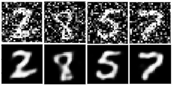
- 노이즈 적용된 검증 데이터
f, ax = plt.subplots(1,5)
f.set_size_inches(80, 40)
for i in range(5,10):
    ax[i-5].imshow(val_x_n[i].reshape(28, 28))
plt.show()

- 노이즈를 없앤 오토인코딩 후 검증 데이터
preds = model_2.predict(val_x_n[:10])
f, ax = plt.subplots(1,5)
f.set_size_inches(80, 40)
for i in range(5,10):
    ax[i-5].imshow(preds[i].reshape(28, 28))
plt.show()

여기서는 적은 epoch로 시도했기에 비교적 불충분한 결과가 나올 수 있지만, 500~1000 epoch 정도로 시도하면 더 좋은 결과가 나올 것입니다.
2.3 UseCase 3: Sequence to Sequence Prediction using AutoEncoders
이번 케이스는 sequence to sequence 예측입니다. 앞의 예시에서는 기본적으로 2차원 데이터였고, 이번에는 sequence 데이터는 1차원 데이터입니다.
이런 시퀀스 데이터의 예시에는 시계열 데이터와 문자열 데이터가 있습니다. 이 예시는 기계 번역 등에 적용할 수 있습니다. 이미지에 CNN을 사용했다면, 이 케이스에서는 LSTM을 사용합니다.
대부분의 코드는 아래의 글에서 참조했다고 합니다.
Most of the code of this section is taken from the following reference shared by Jason Brownie in his blog post. Big Credits to him.
Reference : https://machinelearningmastery.com/develop-encoder-decoder-model-sequence-sequence-prediction-keras/
Autoencoder Architecture
이 케이스의 오토인코더에서도 입력을 변환하는 인코더와 타겟으로 변환하는 디코더가 존재할 것입니다. 우선 LSTM이 이 구조에서 어떤식으로 작동하는지 알아봅시다.
- Long Short-Term Memory, LSTM은 내부 루프로 구성된 반복적 신경망입니다.(RNN)
- 다른 RNN과 다르게 backpropagation throught time, BPTT를 활용하여 효과적으로 훈련하고, 사라지는 그래디언트 문제를 방지합니다.
- LSTM layer에서 메모리 유닛을 정의할 수 있고, layer에 속하지 않은 각 유닛은 셀의 상태를 나타내는 c와 숨겨진 상태이자 출력인 h 등이 있습니다.
- Keras를 사용하면, LSTM 레이어의 출력 상태와 LSTM 레이어의 현재 상태에 모두 접근 할 수 있습니다.
이제 학습과 생성을 하는 오토인코더 구조를 만들어봅시다. 2가지의 요소로 이루어집니다.
- 시퀀스를 입력으로 받아들이고 LSTM의 현재 상태를 출력으로 반환하는 인코더 아키텍처
- 시퀀스 및 인코더 LSTM 상태를 입력으로 받아 디코딩 된 출력 시퀀스를 반환하는 디코더 아키텍처
- LSTM의 숨겨진 상태와 메모리 상태를 저장하고 (숨겨진 그리고 상태들을) 접근하므로,보이지 않는 데이터에 대한 예측을 생성하는 동안 LSTM을 사용할 수 있습니다.
우선, 고정 길이의 무작위 시퀀스를 포함하는 시퀀스 데이터 세트를 생성합니다. 우리는 무작위 순서를 생성하는 함수를 생성 할 것입니다.
- X1은 난수를 포함하는 입력 시퀀스 의미합니다.
- X2는 시퀀스의 다른 요소를 재생산하기 위해 시드로 사용되는 패딩 된 시퀀스를 의미합니다.
- y는 대상 시퀀스 또는 실제 시퀀스를 나타냅니다.
def dataset_preparation(n_in, n_out, n_unique, n_samples):
    X1, X2, y = [], [], []
    for _ in range(n_samples):
        ## create random numbers sequence - input
        inp_seq = [randint(1, n_unique-1) for _ in range(n_in)]

        ## create target sequence
        target = inp_seq[:n_out]

        ## create padded sequence / seed sequence
        target_seq = list(reversed(target))
        seed_seq = [0] + target_seq[:-1]

        # convert the elements to categorical using keras api
        X1.append(to_categorical([inp_seq], num_classes=n_unique))
        X2.append(to_categorical([seed_seq], num_classes=n_unique))
        y.append(to_categorical([target_seq], num_classes=n_unique))

    # remove unnecessary dimention
    X1 = np.squeeze(np.array(X1), axis=1)
    X2 = np.squeeze(np.array(X2), axis=1)
    y  = np.squeeze(np.array(y), axis=1)
    return X1, X2, y

samples = 100000
features = 51
inp_size = 6
out_size = 3

inputs, seeds, outputs = dataset_preparation(inp_size, out_size, features, samples)
print("Shapes: ", inputs.shape, seeds.shape, outputs.shape)
print ("Here is first categorically encoded input sequence looks like: ", )
inputs[0][0]
Shapes:  (100000, 6, 51) (100000, 3, 51) (100000, 3, 51)
Here is first categorically encoded input sequence looks like:
array([0., 0., 0., 0., 0., 0., 0., 0., 0., 0., 1., 0., 0., 0., 0., 0., 0.,
       0., 0., 0., 0., 0., 0., 0., 0., 0., 0., 0., 0., 0., 0., 0., 0., 0.,
       0., 0., 0., 0., 0., 0., 0., 0., 0., 0., 0., 0., 0., 0., 0., 0., 0.],
      dtype=float32)
이제 케라스에서 모델을 만들어봅시다.
def define_models(n_input, n_output):
    ## define the encoder architecture
    ## input : sequence
    ## output : encoder states
    encoder_inputs = Input(shape=(None, n_input))
    encoder = LSTM(128, return_state=True)
    encoder_outputs, state_h, state_c = encoder(encoder_inputs)
    encoder_states = [state_h, state_c]

    ## define the encoder-decoder architecture
    ## input : a seed sequence
    ## output : decoder states, decoded output
    decoder_inputs = Input(shape=(None, n_output))
    decoder_lstm = LSTM(128, return_sequences=True, return_state=True)
    decoder_outputs, _, _ = decoder_lstm(decoder_inputs, initial_state=encoder_states)
    decoder_dense = Dense(n_output, activation='softmax')
    decoder_outputs = decoder_dense(decoder_outputs)
    model = Model([encoder_inputs, decoder_inputs], decoder_outputs)

    ## define the decoder model
    ## input : current states + encoded sequence
    ## output : decoded sequence
    encoder_model = Model(encoder_inputs, encoder_states)
    decoder_state_input_h = Input(shape=(128,))
    decoder_state_input_c = Input(shape=(128,))
    decoder_states_inputs = [decoder_state_input_h, decoder_state_input_c]
    decoder_outputs, state_h, state_c = decoder_lstm(decoder_inputs, initial_state=decoder_states_inputs)
    decoder_states = [state_h, state_c]
    decoder_outputs = decoder_dense(decoder_outputs)
    decoder_model = Model([decoder_inputs] + decoder_states_inputs, [decoder_outputs] + decoder_states)

    return model, encoder_model, decoder_model

autoencoder, encoder_model, decoder_model = define_models(features, features)
각 모델을 확인하면 다음과 같습니다.
encoder_model.summary()
_________________________________________________________________
Layer (type)                 Output Shape              Param #
=================================================================
input_3 (InputLayer)         (None, None, 51)          0
_________________________________________________________________
lstm_1 (LSTM)                [(None, 128), (None, 128) 92160
=================================================================
Total params: 92,160
Trainable params: 92,160
Non-trainable params: 0
_________________________________________________________________
decoder_model.summary()
__________________________________________________________________________________________________
Layer (type)                    Output Shape         Param #     Connected to
==================================================================================================
input_4 (InputLayer)            (None, None, 51)     0
__________________________________________________________________________________________________
input_5 (InputLayer)            (None, 128)          0
__________________________________________________________________________________________________
input_6 (InputLayer)            (None, 128)          0
__________________________________________________________________________________________________
lstm_2 (LSTM)                   [(None, None, 128),  92160       input_4[0][0]
                                                                 input_5[0][0]
                                                                 input_6[0][0]
__________________________________________________________________________________________________
dense_9 (Dense)                 (None, None, 51)     6579        lstm_2[1][0]
==================================================================================================
Total params: 98,739
Trainable params: 98,739
Non-trainable params: 0
__________________________________________________________________________________________________
autoencoder.summary()
__________________________________________________________________________________________________
Layer (type)                    Output Shape         Param #     Connected to
==================================================================================================
input_3 (InputLayer)            (None, None, 51)     0
__________________________________________________________________________________________________
input_4 (InputLayer)            (None, None, 51)     0
__________________________________________________________________________________________________
lstm_1 (LSTM)                   [(None, 128), (None, 92160       input_3[0][0]
__________________________________________________________________________________________________
lstm_2 (LSTM)                   [(None, None, 128),  92160       input_4[0][0]
                                                                 lstm_1[0][1]
                                                                 lstm_1[0][2]
__________________________________________________________________________________________________
dense_9 (Dense)                 (None, None, 51)     6579        lstm_2[0][0]
==================================================================================================
Total params: 190,899
Trainable params: 190,899
Non-trainable params: 0
__________________________________________________________________________________________________
이제 오토인코더 모델을 아담 옵티마이저와 Catgegorical Cross Entropy를 손실함수로 사용하여 훈련해봅시다.
autoencoder.compile(optimizer='adam', loss='categorical_crossentropy', metrics=['acc'])
autoencoder.fit([inputs, seeds], outputs, epochs=1)
Epoch 1/1
100000/100000 [==============================] - 41s 412us/step - loss: 0.6398 - acc: 0.7950
<keras.callbacks.History at 0x7f12ec2119b0>
이제 입력 시퀀스를 이용해 시퀀스를 예측하는 함수를 만들어봅시다.
def reverse_onehot(encoded_seq):
    return [argmax(vector) for vector in encoded_seq]

def predict_sequence(encoder, decoder, sequence):
    output = []
    target_seq = np.array([0.0 for _ in range(features)])
    target_seq = target_seq.reshape(1, 1, features)

    current_state = encoder.predict(sequence)
    for t in range(out_size):
        pred, h, c = decoder.predict([target_seq] + current_state)
        output.append(pred[0, 0, :])
        current_state = [h, c]
        target_seq = pred
    return np.array(output)
이제 예측을 만들어 봅시다.
for k in range(5):
    X1, X2, y = dataset_preparation(inp_size, out_size, features, 1)
    target = predict_sequence(encoder_model, decoder_model, X1)
    print('\nInput Sequence=%s SeedSequence=%s, PredictedSequence=%s'
          % (reverse_onehot(X1[0]), reverse_onehot(y[0]), reverse_onehot(target)))
Input Sequence=[32, 18, 28, 22, 40, 17] SeedSequence=[28, 18, 32], PredictedSequence=[28, 18, 32]

Input Sequence=[43, 36, 33, 37, 27, 21] SeedSequence=[33, 36, 43], PredictedSequence=[33, 36, 43]

Input Sequence=[10, 14, 49, 44, 5, 36] SeedSequence=[49, 14, 10], PredictedSequence=[49, 14, 10]

Input Sequence=[28, 13, 44, 9, 30, 24] SeedSequence=[44, 13, 28], PredictedSequence=[44, 13, 28]

Input Sequence=[35, 35, 37, 9, 2, 4] SeedSequence=[37, 35, 35], PredictedSequence=[37, 35, 35]
Excellent References
- https://www.analyticsvidhya.com/blog/2018/06/unsupervised-deep-learning-computer-vision/
- https://towardsdatascience.com/applied-deep-learning-part-3-autoencoders-1c083af4d798
- https://blog.keras.io/building-autoencoders-in-keras.html
- https://cs.stanford.edu/people/karpathy/convnetjs/demo/autoencoder.html
- https://machinelearningmastery.com/develop-encoder-decoder-model-sequence-sequence-prediction-keras/
마지막으로 이렇게 좋은 커널을 만들어주신 @ShivamBansal님에게 다시 한번 감사의 인사를 드립니다.
Finally, thanks to @ShivamBansal for making such a good kernel.