본 커널은 @thebrownviking님의 Everything you can do with a time series을 번역한 커널입니다.
최종 업데이트 : 2019.05.21
Aim
이 플랫폼을 시작한 첫 주부터 저는 시계열 분석이라는 주제에 매료되었습니다. 이 커널을 시계열 분석에서 다양한 주제를 다루기 위해 만든 커널입니다. 저는 시계열 분석에서 초보자와 숙련자 모두에게 ultimate reference(궁극적 레퍼런스)를 만들고 싶었습니다.
Some important things
- 이 커널은 현재진행형으로, home feed에서 볼 때마다 새로운 컨텐츠를 확인하실 수 있을 것입니다.
- 다양한 과정을 마친 후, 이 분야에 집중하고 있습니다. advanced한 내용을 전달하기 위해 더 연구하고 있습니다.
- 특정 주제에 대한 제안은 친절한 댓글을 통해 부탁드립니다.
- 만약 이 커널이 도움이 됬다면 커널에 upvote를 눌러주세요.
역자의 말
안수빈(@subinium) 이 번역한 커널입니다.
- 일부 단어는 그 의미를 살리기 위해 번역하지 않고 사용했습니다.
- 소제목은 의미를 더 확실하게 전하기 위해 원문을 그대로 가져왔습니다.
- 메서드나 주제에서 설명이 부족한 경우, 추가한 내용이 있습니다.
- 모델 부분은 설명이 부족하고, 코드에 대한 주석이 없어 이해가 힘들 수 있습니다.
- 상태 공간 모델의 경우, 제가 시계열 분석에 대한 이해가 부족해 더 자세하게 번역하지 못했습니다.
# Importing libraries
import os
import warnings
warnings.filterwarnings('ignore')
import numpy as np
import pandas as pd
import matplotlib.pyplot as plt
plt.style.use('fivethirtyeight')
# Above is a special style template for matplotlib, highly useful for visualizing time series data
%matplotlib inline
from pylab import rcParams
from plotly import tools
import plotly.plotly as py
from plotly.offline import init_notebook_mode, iplot
init_notebook_mode(connected=True)
import plotly.graph_objs as go
import plotly.figure_factory as ff
import statsmodels.api as sm
from numpy.random import normal, seed
from scipy.stats import norm
from statsmodels.tsa.arima_model import ARMA
from statsmodels.tsa.stattools import adfuller
from statsmodels.graphics.tsaplots import plot_acf, plot_pacf
from statsmodels.tsa.arima_process import ArmaProcess
from statsmodels.tsa.arima_model import ARIMA
import math
from sklearn.metrics import mean_squared_error
print(os.listdir("../input"))
['stock-time-series-20050101-to-20171231', 'historical-hourly-weather-data']
How to import data?
우선 이 커널에서 필요한 데이터셋을 불러와야합니다. pd.read_csv()에서 두 개의 매개변수를 사용해서 불러옵시다.
- parse_dates 매개변수를 사용하여 필요한 시계열을 datetime 열로 변환합니다.
- dataframe의 index는 index_col로 지정합니다.
아래 코드를 보면 더 이해가 쉬울 것입니다.
Data being used:-
사용하는 데이터는 다음과 같습니다.
- Google Stocks Data (구글 주식 데이터)
- Humidity in different world cities (세계 여러 도시의 습도 데이터)
- Microsoft Stocks Data (마이크로소프트 주식 데이터)
- Pressure in different world cities (세계 여러 도시의 기압 데이터)
google = pd.read_csv('../input/stock-time-series-20050101-to-20171231/GOOGL_2006-01-01_to_2018-01-01.csv', index_col='Date', parse_dates=['Date'])
google.head()
| Open | High | Low | Close | Volume | Name | |
|---|---|---|---|---|---|---|
| Date | ||||||
| 2006-01-03 | 211.47 | 218.05 | 209.32 | 217.83 | 13137450 | GOOGL |
| 2006-01-04 | 222.17 | 224.70 | 220.09 | 222.84 | 15292353 | GOOGL |
| 2006-01-05 | 223.22 | 226.00 | 220.97 | 225.85 | 10815661 | GOOGL |
| 2006-01-06 | 228.66 | 235.49 | 226.85 | 233.06 | 17759521 | GOOGL |
| 2006-01-09 | 233.44 | 236.94 | 230.70 | 233.68 | 12795837 | GOOGL |
humidity = pd.read_csv('../input/historical-hourly-weather-data/humidity.csv', index_col='datetime', parse_dates=['datetime'])
humidity.tail()
| Vancouver | Portland | San Francisco | Seattle | Los Angeles | San Diego | Las Vegas | Phoenix | Albuquerque | Denver | San Antonio | Dallas | Houston | Kansas City | Minneapolis | Saint Louis | Chicago | Nashville | Indianapolis | Atlanta | Detroit | Jacksonville | Charlotte | Miami | Pittsburgh | Toronto | Philadelphia | New York | Montreal | Boston | Beersheba | Tel Aviv District | Eilat | Haifa | Nahariyya | Jerusalem | |
|---|---|---|---|---|---|---|---|---|---|---|---|---|---|---|---|---|---|---|---|---|---|---|---|---|---|---|---|---|---|---|---|---|---|---|---|---|
| datetime | ||||||||||||||||||||||||||||||||||||
| 2017-11-29 20:00:00 | NaN | 81.0 | NaN | 93.0 | 24.0 | 72.0 | 18.0 | 68.0 | 37.0 | 18.0 | 37.0 | 45.0 | 68.0 | 32.0 | 31.0 | 32.0 | 52.0 | 32.0 | 32.0 | 82.0 | 39.0 | 47.0 | 21.0 | NaN | 20.0 | 45.0 | 27.0 | NaN | 64.0 | 37.0 | NaN | NaN | NaN | NaN | NaN | NaN |
| 2017-11-29 21:00:00 | NaN | 71.0 | NaN | 87.0 | 21.0 | 72.0 | 18.0 | 73.0 | 34.0 | 12.0 | 35.0 | 42.0 | 73.0 | 27.0 | 31.0 | 37.0 | 65.0 | 34.0 | 32.0 | 73.0 | 39.0 | 47.0 | 21.0 | NaN | 23.0 | 48.0 | 29.0 | NaN | 59.0 | 74.0 | NaN | NaN | NaN | NaN | NaN | NaN |
| 2017-11-29 22:00:00 | NaN | 71.0 | NaN | 93.0 | 23.0 | 68.0 | 17.0 | 60.0 | 32.0 | 15.0 | 38.0 | 42.0 | 50.0 | 27.0 | 30.0 | 37.0 | 96.0 | 36.0 | 39.0 | 77.0 | 42.0 | 53.0 | 24.0 | NaN | 27.0 | 52.0 | 31.0 | NaN | 66.0 | 74.0 | NaN | NaN | NaN | NaN | NaN | NaN |
| 2017-11-29 23:00:00 | NaN | 71.0 | NaN | 87.0 | 14.0 | 63.0 | 17.0 | 33.0 | 30.0 | 28.0 | 37.0 | 45.0 | 49.0 | 30.0 | 35.0 | 46.0 | 75.0 | 39.0 | 52.0 | 82.0 | 52.0 | 73.0 | 38.0 | NaN | 36.0 | 64.0 | 26.0 | NaN | 58.0 | 56.0 | NaN | NaN | NaN | NaN | NaN | NaN |
| 2017-11-30 00:00:00 | NaN | 76.0 | NaN | 75.0 | 56.0 | 72.0 | 17.0 | 23.0 | 34.0 | 31.0 | 48.0 | 42.0 | 52.0 | 32.0 | 38.0 | 46.0 | 86.0 | 41.0 | 52.0 | 100.0 | 56.0 | 88.0 | 41.0 | NaN | 42.0 | 60.0 | 32.0 | NaN | 58.0 | 56.0 | NaN | NaN | NaN | NaN | NaN | NaN |
How to prepare data?
구글 주식 데이터는 누락 데이터가 없지만, 습도 데이터는 누락데이터가 꽤 있습니다.
누락 데이터는 fillna() 메서드와 ffill 매개변수를 이용해 채웁니다. fillna()의 매개변수는 다음과 같은 매개변수가 있습니다. 이는 후에도 언급하니 가볍게 넘어가면 될 것 같습니다.
- ffill : 앞의 값을 관찰한 값으로 채워넣음
- bfill : 뒤의 값을 관찰한 값으로 채워넣음
humidity = humidity.iloc[1:]
humidity = humidity.fillna(method='ffill')
humidity.head()
| Vancouver | Portland | San Francisco | Seattle | Los Angeles | San Diego | Las Vegas | Phoenix | Albuquerque | Denver | San Antonio | Dallas | Houston | Kansas City | Minneapolis | Saint Louis | Chicago | Nashville | Indianapolis | Atlanta | Detroit | Jacksonville | Charlotte | Miami | Pittsburgh | Toronto | Philadelphia | New York | Montreal | Boston | Beersheba | Tel Aviv District | Eilat | Haifa | Nahariyya | Jerusalem | |
|---|---|---|---|---|---|---|---|---|---|---|---|---|---|---|---|---|---|---|---|---|---|---|---|---|---|---|---|---|---|---|---|---|---|---|---|---|
| datetime | ||||||||||||||||||||||||||||||||||||
| 2012-10-01 13:00:00 | 76.0 | 81.0 | 88.0 | 81.0 | 88.0 | 82.0 | 22.0 | 23.0 | 50.0 | 62.0 | 93.0 | 87.0 | 93.0 | 71.0 | 67.0 | 71.0 | 71.0 | 100.0 | 76.0 | 94.0 | 76.0 | 88.0 | 87.0 | 83.0 | 93.0 | 82.0 | 71.0 | 58.0 | 93.0 | 68.0 | 50.0 | 63.0 | 22.0 | 51.0 | 51.0 | 50.0 |
| 2012-10-01 14:00:00 | 76.0 | 80.0 | 87.0 | 80.0 | 88.0 | 81.0 | 21.0 | 23.0 | 49.0 | 62.0 | 92.0 | 86.0 | 92.0 | 70.0 | 66.0 | 71.0 | 70.0 | 99.0 | 76.0 | 94.0 | 75.0 | 87.0 | 87.0 | 82.0 | 93.0 | 81.0 | 70.0 | 57.0 | 91.0 | 68.0 | 51.0 | 62.0 | 22.0 | 51.0 | 51.0 | 50.0 |
| 2012-10-01 15:00:00 | 76.0 | 80.0 | 86.0 | 80.0 | 88.0 | 81.0 | 21.0 | 23.0 | 49.0 | 62.0 | 92.0 | 86.0 | 90.0 | 70.0 | 66.0 | 71.0 | 70.0 | 99.0 | 76.0 | 94.0 | 75.0 | 87.0 | 87.0 | 82.0 | 93.0 | 79.0 | 70.0 | 57.0 | 87.0 | 68.0 | 51.0 | 62.0 | 22.0 | 51.0 | 51.0 | 50.0 |
| 2012-10-01 16:00:00 | 77.0 | 80.0 | 85.0 | 79.0 | 88.0 | 81.0 | 21.0 | 23.0 | 49.0 | 62.0 | 92.0 | 86.0 | 89.0 | 70.0 | 65.0 | 71.0 | 70.0 | 99.0 | 76.0 | 94.0 | 74.0 | 87.0 | 87.0 | 82.0 | 93.0 | 77.0 | 69.0 | 57.0 | 84.0 | 68.0 | 52.0 | 62.0 | 22.0 | 51.0 | 51.0 | 50.0 |
| 2012-10-01 17:00:00 | 78.0 | 79.0 | 84.0 | 79.0 | 88.0 | 80.0 | 21.0 | 24.0 | 49.0 | 63.0 | 92.0 | 86.0 | 88.0 | 69.0 | 65.0 | 71.0 | 69.0 | 99.0 | 76.0 | 94.0 | 74.0 | 86.0 | 87.0 | 81.0 | 93.0 | 76.0 | 69.0 | 57.0 | 80.0 | 68.0 | 54.0 | 62.0 | 23.0 | 51.0 | 51.0 | 50.0 |
asfreq 메서드는 시계열을 특정 frequency로 변환합니다. (30S = 30초, M = 매월)
upsampling 또는 downsampling에 사용할 수 있습니다.
여기서는 매개변수를 'M'으로 전달하였고, 이는 매월 빈도를 의미합니다.
humidity["Kansas City"].asfreq('M').plot() # asfreq method is used to convert a time series to a specified frequency. Here it is monthly frequency.
plt.title('Humidity in Kansas City over time(Monthly frequency)')
plt.show()

google['2008':'2010'].plot(subplots=True, figsize=(10,12))
plt.title('Google stock attributes from 2008 to 2010')
plt.savefig('stocks.png')
plt.show()

What are timestamps and periods and how are they useful?
timestamp와 period는 무엇이고, 어떻게 유용할까요?
Timestamp는 특정 시점을 나타내기 위해 사용됩니다.
Period는 특정 기간을 나타내기 위해 사용됩니다.
Periods는 기간동안 특정 이벤트가 있는지 체크하는데 사용할 수 있습니다. 각각은 서로 변환가능합니다. 우선 아래 예시로 생성 방법을 살펴보겠습니다.
# Creating a Timestamp
timestamp = pd.Timestamp(2017, 1, 1, 12)
timestamp
Timestamp('2017-01-01 12:00:00')
# Creating a period
period = pd.Period('2017-01-01')
period
Period('2017-01-01', 'D')
timestamp와 period는 이런 비교가 가능합니다.
# Checking if the given timestamp exists in the given period
period.start_time < timestamp < period.end_time
True
변환의 예시는 다음과 같습니다.
# Converting timestamp to period
new_period = timestamp.to_period(freq='H')
new_period
Period('2017-01-01 12:00', 'H')
# Converting period to timestamp
new_timestamp = period.to_timestamp(freq='H', how='start')
new_timestamp
Timestamp('2017-01-01 00:00:00')
What is date_range and how is it useful?
date_range는 무엇이고, 어떻게 유용할까요?
date_range는 고정 frequency datetimeindex를 반환하는 메서드입니다. 이것도 예시를 봐야 이해가 빠를 것 같습니다.
이는 기존 데이터에서 본인만의 시계열 요소를 만들거나 전체 데이터를 정리(arranging)하는데 사용할 수 있습니다.
# Creating a datetimeindex with daily frequency
dr1 = pd.date_range(start='1/1/18', end='1/9/18')
dr1
DatetimeIndex(['2018-01-01', '2018-01-02', '2018-01-03', '2018-01-04',
'2018-01-05', '2018-01-06', '2018-01-07', '2018-01-08',
'2018-01-09'],
dtype='datetime64[ns]', freq='D')
# Creating a datetimeindex with monthly frequency
dr2 = pd.date_range(start='1/1/18', end='1/1/19', freq='M')
dr2
DatetimeIndex(['2018-01-31', '2018-02-28', '2018-03-31', '2018-04-30',
'2018-05-31', '2018-06-30', '2018-07-31', '2018-08-31',
'2018-09-30', '2018-10-31', '2018-11-30', '2018-12-31'],
dtype='datetime64[ns]', freq='M')
아래와 같이 시작과 종료 시점 중 하나만 있어도 되고, 원하는 period에서 시계열을 만들 수 있습니다.
# Creating a datetimeindex without specifying start date and using periods
dr3 = pd.date_range(end='1/4/2014', periods=8)
dr3
DatetimeIndex(['2013-12-28', '2013-12-29', '2013-12-30', '2013-12-31',
'2014-01-01', '2014-01-02', '2014-01-03', '2014-01-04'],
dtype='datetime64[ns]', freq='D')
# Creating a datetimeindex specifying start date , end date and periods
dr4 = pd.date_range(start='2013-04-24', end='2014-11-27', periods=3)
dr4
DatetimeIndex(['2013-04-24', '2014-02-09', '2014-11-27'], dtype='datetime64[ns]', freq=None)
pandas.to_datetime()은 Dataframe을 datetime으로 변환하는 함수입니다.
df = pd.DataFrame({'year': [2015, 2016], 'month': [2, 3], 'day': [4, 5]})
df
| year | month | day | |
|---|---|---|---|
| 0 | 2015 | 2 | 4 |
| 1 | 2016 | 3 | 5 |
df = pd.to_datetime(df)
df
0 2015-02-04 1 2016-03-05 dtype: datetime64[ns]
df = pd.to_datetime('01-01-2017')
df
Timestamp('2017-01-01 00:00:00')
우리는 원하는 기간을 shift하여 index를 원하는 frequency로 이동변환 가능합니다.
이는 과거와 현재의 시계열을 비교하는데 유용합니다.
아래는 데이터를 월 단위로 바꾼 후에 10개월을 shift한 후 시각화한 그래프입니다.
humidity["Vancouver"].asfreq('M').plot(legend=True)
shifted = humidity["Vancouver"].asfreq('M').shift(10).plot(legend=True)
shifted.legend(['Vancouver','Vancouver_lagged'])
plt.show()

1.8 Resampling
Upsampling : 시계열을 low frequency에서 high frequency로 변환(리샘플링)합니다. 누락된 데이터를 채우거나 보간하는 방법을 포함합니다. (월 데이터 -> 일 데이터)
Downsampling : 시계열을 high frequency에서 low frequency로 변환(리샘플링)합니다. 기존 데이터를 집계하는 것을 포함합니다. (주간 데이터 -> 월 데이터)
# Let's use pressure data to demonstrate this
pressure = pd.read_csv('../input/historical-hourly-weather-data/pressure.csv', index_col='datetime', parse_dates=['datetime'])
pressure.tail()
| Vancouver | Portland | San Francisco | Seattle | Los Angeles | San Diego | Las Vegas | Phoenix | Albuquerque | Denver | San Antonio | Dallas | Houston | Kansas City | Minneapolis | Saint Louis | Chicago | Nashville | Indianapolis | Atlanta | Detroit | Jacksonville | Charlotte | Miami | Pittsburgh | Toronto | Philadelphia | New York | Montreal | Boston | Beersheba | Tel Aviv District | Eilat | Haifa | Nahariyya | Jerusalem | |
|---|---|---|---|---|---|---|---|---|---|---|---|---|---|---|---|---|---|---|---|---|---|---|---|---|---|---|---|---|---|---|---|---|---|---|---|---|
| datetime | ||||||||||||||||||||||||||||||||||||
| 2017-11-29 20:00:00 | NaN | 1031.0 | NaN | 1030.0 | 1016.0 | 1017.0 | 1021.0 | 1018.0 | 1025.0 | 1016.0 | 1022.0 | 1021.0 | 1021.0 | 1020.0 | 1018.0 | 1023.0 | 1025.0 | 1023.0 | 1025.0 | 1024.0 | 1027.0 | 1021.0 | 1023.0 | NaN | 1024.0 | 1026.0 | 1021.0 | NaN | 1021.0 | 1017.0 | NaN | NaN | NaN | NaN | NaN | NaN |
| 2017-11-29 21:00:00 | NaN | 1030.0 | NaN | 1030.0 | 1016.0 | 1017.0 | 1020.0 | 1018.0 | 1024.0 | 1018.0 | 1021.0 | 1021.0 | 1021.0 | 1021.0 | 1017.0 | 1022.0 | 1024.0 | 1022.0 | 1024.0 | 1023.0 | 1027.0 | 1021.0 | 1023.0 | NaN | 1024.0 | 1026.0 | 1021.0 | NaN | 1023.0 | 1019.0 | NaN | NaN | NaN | NaN | NaN | NaN |
| 2017-11-29 22:00:00 | NaN | 1030.0 | NaN | 1029.0 | 1015.0 | 1016.0 | 1020.0 | 1017.0 | 1024.0 | 1018.0 | 1021.0 | 1021.0 | 1020.0 | 1020.0 | 1016.0 | 1021.0 | 1024.0 | 1023.0 | 1024.0 | 1023.0 | 1027.0 | 1022.0 | 1023.0 | NaN | 1024.0 | 1026.0 | 1022.0 | NaN | 1024.0 | 1019.0 | NaN | NaN | NaN | NaN | NaN | NaN |
| 2017-11-29 23:00:00 | NaN | 1029.0 | NaN | 1028.0 | 1016.0 | 1016.0 | 1020.0 | 1016.0 | 1024.0 | 1020.0 | 1021.0 | 1021.0 | 1020.0 | 1019.0 | 1015.0 | 1021.0 | 1023.0 | 1023.0 | 1024.0 | 1023.0 | 1027.0 | 1022.0 | 1023.0 | NaN | 1024.0 | 1027.0 | 1023.0 | NaN | 1026.0 | 1022.0 | NaN | NaN | NaN | NaN | NaN | NaN |
| 2017-11-30 00:00:00 | NaN | 1029.0 | NaN | 1028.0 | 1015.0 | 1017.0 | 1019.0 | 1016.0 | 1024.0 | 1021.0 | 1021.0 | 1021.0 | 1020.0 | 1019.0 | 1016.0 | 1021.0 | 1023.0 | 1023.0 | 1023.0 | 1024.0 | 1027.0 | 1022.0 | 1024.0 | NaN | 1025.0 | 1027.0 | 1024.0 | NaN | 1027.0 | 1023.0 | NaN | NaN | NaN | NaN | NaN | NaN |
시작부터 채워야하는 데이터들이 보입니다. 이는 다음과 같이 채울 수 있습니다.
pressure = pressure.iloc[1:]
pressure = pressure.fillna(method='ffill')
pressure.tail()
| Vancouver | Portland | San Francisco | Seattle | Los Angeles | San Diego | Las Vegas | Phoenix | Albuquerque | Denver | San Antonio | Dallas | Houston | Kansas City | Minneapolis | Saint Louis | Chicago | Nashville | Indianapolis | Atlanta | Detroit | Jacksonville | Charlotte | Miami | Pittsburgh | Toronto | Philadelphia | New York | Montreal | Boston | Beersheba | Tel Aviv District | Eilat | Haifa | Nahariyya | Jerusalem | |
|---|---|---|---|---|---|---|---|---|---|---|---|---|---|---|---|---|---|---|---|---|---|---|---|---|---|---|---|---|---|---|---|---|---|---|---|---|
| datetime | ||||||||||||||||||||||||||||||||||||
| 2017-11-29 20:00:00 | 1021.0 | 1031.0 | 1013.0 | 1030.0 | 1016.0 | 1017.0 | 1021.0 | 1018.0 | 1025.0 | 1016.0 | 1022.0 | 1021.0 | 1021.0 | 1020.0 | 1018.0 | 1023.0 | 1025.0 | 1023.0 | 1025.0 | 1024.0 | 1027.0 | 1021.0 | 1023.0 | 1015.0 | 1024.0 | 1026.0 | 1021.0 | 1020.0 | 1021.0 | 1017.0 | 984.0 | 1011.0 | 968.0 | 1023.0 | 1023.0 | 1011.0 |
| 2017-11-29 21:00:00 | 1021.0 | 1030.0 | 1013.0 | 1030.0 | 1016.0 | 1017.0 | 1020.0 | 1018.0 | 1024.0 | 1018.0 | 1021.0 | 1021.0 | 1021.0 | 1021.0 | 1017.0 | 1022.0 | 1024.0 | 1022.0 | 1024.0 | 1023.0 | 1027.0 | 1021.0 | 1023.0 | 1015.0 | 1024.0 | 1026.0 | 1021.0 | 1020.0 | 1023.0 | 1019.0 | 984.0 | 1011.0 | 968.0 | 1023.0 | 1023.0 | 1011.0 |
| 2017-11-29 22:00:00 | 1021.0 | 1030.0 | 1013.0 | 1029.0 | 1015.0 | 1016.0 | 1020.0 | 1017.0 | 1024.0 | 1018.0 | 1021.0 | 1021.0 | 1020.0 | 1020.0 | 1016.0 | 1021.0 | 1024.0 | 1023.0 | 1024.0 | 1023.0 | 1027.0 | 1022.0 | 1023.0 | 1015.0 | 1024.0 | 1026.0 | 1022.0 | 1020.0 | 1024.0 | 1019.0 | 984.0 | 1011.0 | 968.0 | 1023.0 | 1023.0 | 1011.0 |
| 2017-11-29 23:00:00 | 1021.0 | 1029.0 | 1013.0 | 1028.0 | 1016.0 | 1016.0 | 1020.0 | 1016.0 | 1024.0 | 1020.0 | 1021.0 | 1021.0 | 1020.0 | 1019.0 | 1015.0 | 1021.0 | 1023.0 | 1023.0 | 1024.0 | 1023.0 | 1027.0 | 1022.0 | 1023.0 | 1015.0 | 1024.0 | 1027.0 | 1023.0 | 1020.0 | 1026.0 | 1022.0 | 984.0 | 1011.0 | 968.0 | 1023.0 | 1023.0 | 1011.0 |
| 2017-11-30 00:00:00 | 1021.0 | 1029.0 | 1013.0 | 1028.0 | 1015.0 | 1017.0 | 1019.0 | 1016.0 | 1024.0 | 1021.0 | 1021.0 | 1021.0 | 1020.0 | 1019.0 | 1016.0 | 1021.0 | 1023.0 | 1023.0 | 1023.0 | 1024.0 | 1027.0 | 1022.0 | 1024.0 | 1015.0 | 1025.0 | 1027.0 | 1024.0 | 1020.0 | 1027.0 | 1023.0 | 984.0 | 1011.0 | 968.0 | 1023.0 | 1023.0 | 1011.0 |
pressure = pressure.fillna(method='bfill')
pressure.head()
| Vancouver | Portland | San Francisco | Seattle | Los Angeles | San Diego | Las Vegas | Phoenix | Albuquerque | Denver | San Antonio | Dallas | Houston | Kansas City | Minneapolis | Saint Louis | Chicago | Nashville | Indianapolis | Atlanta | Detroit | Jacksonville | Charlotte | Miami | Pittsburgh | Toronto | Philadelphia | New York | Montreal | Boston | Beersheba | Tel Aviv District | Eilat | Haifa | Nahariyya | Jerusalem | |
|---|---|---|---|---|---|---|---|---|---|---|---|---|---|---|---|---|---|---|---|---|---|---|---|---|---|---|---|---|---|---|---|---|---|---|---|---|
| datetime | ||||||||||||||||||||||||||||||||||||
| 2012-10-01 13:00:00 | 807.0 | 1024.0 | 1009.0 | 1027.0 | 1013.0 | 1013.0 | 1018.0 | 1013.0 | 1024.0 | 1028.0 | 1014.0 | 1011.0 | 1009.0 | 1011.0 | 1012.0 | 1010.0 | 1014.0 | 1005.0 | 1011.0 | 1006.0 | 1016.0 | 1009.0 | 1012.0 | 1011.0 | 1015.0 | 1012.0 | 1014.0 | 1012.0 | 1001.0 | 1014.0 | 984.0 | 1012.0 | 1010.0 | 1013.0 | 1013.0 | 990.0 |
| 2012-10-01 14:00:00 | 807.0 | 1024.0 | 1009.0 | 1027.0 | 1013.0 | 1013.0 | 1018.0 | 1013.0 | 1024.0 | 1028.0 | 1014.0 | 1011.0 | 1008.0 | 1011.0 | 1012.0 | 1010.0 | 1014.0 | 1004.0 | 1011.0 | 1006.0 | 1015.0 | 1009.0 | 1012.0 | 1011.0 | 1015.0 | 1011.0 | 1014.0 | 1012.0 | 986.0 | 1014.0 | 984.0 | 1012.0 | 1010.0 | 1013.0 | 1013.0 | 990.0 |
| 2012-10-01 15:00:00 | 807.0 | 1024.0 | 1009.0 | 1028.0 | 1013.0 | 1013.0 | 1018.0 | 1013.0 | 1024.0 | 1028.0 | 1014.0 | 1011.0 | 1008.0 | 1011.0 | 1012.0 | 1010.0 | 1014.0 | 1004.0 | 1011.0 | 1006.0 | 1015.0 | 1009.0 | 1012.0 | 1011.0 | 1015.0 | 1011.0 | 1014.0 | 1012.0 | 945.0 | 1014.0 | 984.0 | 1012.0 | 1010.0 | 1013.0 | 1013.0 | 990.0 |
| 2012-10-01 16:00:00 | 807.0 | 1024.0 | 1009.0 | 1028.0 | 1013.0 | 1013.0 | 1018.0 | 1013.0 | 1024.0 | 1028.0 | 1014.0 | 1011.0 | 1008.0 | 1011.0 | 1012.0 | 1010.0 | 1014.0 | 1004.0 | 1011.0 | 1006.0 | 1015.0 | 1009.0 | 1012.0 | 1011.0 | 1015.0 | 1010.0 | 1014.0 | 1012.0 | 904.0 | 1014.0 | 984.0 | 1012.0 | 1010.0 | 1013.0 | 1013.0 | 990.0 |
| 2012-10-01 17:00:00 | 807.0 | 1024.0 | 1009.0 | 1029.0 | 1013.0 | 1013.0 | 1018.0 | 1013.0 | 1024.0 | 1028.0 | 1014.0 | 1011.0 | 1008.0 | 1011.0 | 1012.0 | 1010.0 | 1014.0 | 1004.0 | 1011.0 | 1006.0 | 1015.0 | 1009.0 | 1012.0 | 1011.0 | 1015.0 | 1010.0 | 1014.0 | 1012.0 | 863.0 | 1014.0 | 984.0 | 1012.0 | 1010.0 | 1013.0 | 1013.0 | 990.0 |
- ffill 파라미터를 사용하면 마지막 유효 관측치를 전파하여 데이터의 갭을 채웁니다.
- bfill 파라미터를 사용하면 다음 유효 관측치를 전파하여 데이터의 갭을 채웁니다.
# Shape before resampling(downsampling)
pressure.shape
(45252, 36)
기존 데이터는 1시간 단위로 존재했습니다. 이를 3일 단위로 다운샘플링해보겠습니다.
resample 메서드를 사용했고, 평균을 사용했습니다.
# We downsample from hourly to 3 day frequency aggregated using mean
pressure = pressure.resample('3D').mean()
pressure.head()
| Vancouver | Portland | San Francisco | Seattle | Los Angeles | San Diego | Las Vegas | Phoenix | Albuquerque | Denver | San Antonio | Dallas | Houston | Kansas City | Minneapolis | Saint Louis | Chicago | Nashville | Indianapolis | Atlanta | Detroit | Jacksonville | Charlotte | Miami | Pittsburgh | Toronto | Philadelphia | New York | Montreal | Boston | Beersheba | Tel Aviv District | Eilat | Haifa | Nahariyya | Jerusalem | |
|---|---|---|---|---|---|---|---|---|---|---|---|---|---|---|---|---|---|---|---|---|---|---|---|---|---|---|---|---|---|---|---|---|---|---|---|---|
| datetime | ||||||||||||||||||||||||||||||||||||
| 2012-10-01 13:00:00 | 946.652778 | 1022.597222 | 1010.666667 | 1030.666667 | 1011.472222 | 1011.875000 | 1015.305556 | 1011.805556 | 1021.722222 | 1022.347222 | 1014.638889 | 1012.000000 | 1010.750000 | 1012.111111 | 1012.791667 | 1010.166667 | 1012.388889 | 1006.680556 | 1009.680556 | 1008.402778 | 1013.777778 | 1010.652778 | 1012.263889 | 1013.013889 | 1012.902778 | 1005.486111 | 1014.388889 | 1013.875000 | 952.013889 | 1014.291667 | 985.388889 | 1013.277778 | 1012.208333 | 1013.000000 | 1013.000000 | 990.611111 |
| 2012-10-04 13:00:00 | 1018.875000 | 1022.819444 | 1016.027778 | 1027.527778 | 1016.208333 | 1016.888889 | 1013.597222 | 1014.486111 | 1019.930556 | 1022.375000 | 1017.847222 | 1017.361111 | 1017.888889 | 1019.625000 | 1016.750000 | 1020.222222 | 1017.000000 | 1021.069444 | 1019.541667 | 1021.527778 | 1017.430556 | 1019.847222 | 1021.291667 | 1017.847222 | 1018.930556 | 1007.291667 | 1017.763889 | 1017.083333 | 1015.680556 | 1019.555556 | 984.486111 | 1012.791667 | 1012.277778 | 1013.000000 | 1013.000000 | 989.902778 |
| 2012-10-07 13:00:00 | 1014.125000 | 1016.652778 | 1016.527778 | 1017.472222 | 1013.388889 | 1014.347222 | 1012.500000 | 1011.652778 | 1005.875000 | 1018.541667 | 1020.750000 | 1022.583333 | 1019.333333 | 1020.888889 | 1014.652778 | 1022.194444 | 1020.152778 | 1021.652778 | 1021.291667 | 1018.375000 | 1020.277778 | 1015.527778 | 1018.694444 | 1014.097222 | 1020.263889 | 1007.166667 | 1019.666667 | 1018.652778 | 1017.013889 | 1016.805556 | 982.833333 | 1012.902778 | 1007.500000 | 1013.000000 | 1013.000000 | 989.722222 |
| 2012-10-10 13:00:00 | 1011.375000 | 1014.513889 | 1014.416667 | 1017.472222 | 1009.916667 | 1013.750000 | 997.625000 | 1004.125000 | 978.263889 | 977.722222 | 1014.652778 | 1016.138889 | 1017.652778 | 1015.027778 | 1012.583333 | 1019.513889 | 1016.361111 | 1019.194444 | 1017.708333 | 1017.986111 | 1015.597222 | 1019.138889 | 1019.375000 | 1016.513889 | 1014.361111 | 1009.597222 | 1017.958333 | 1016.916667 | 1014.083333 | 1017.652778 | 979.305556 | 1005.847222 | 995.013889 | 1012.333333 | 1012.333333 | 988.013889 |
| 2012-10-13 13:00:00 | 1010.208333 | 1018.694444 | 1021.888889 | 1016.152778 | 1017.972222 | 1018.347222 | 1019.611111 | 1017.527778 | 1022.652778 | 1018.888889 | 1018.291667 | 1016.805556 | 1017.680556 | 1013.527778 | 1012.888889 | 1015.625000 | 1013.916667 | 1020.236111 | 1016.361111 | 1022.638889 | 1016.250000 | 1020.916667 | 1024.708333 | 1016.666667 | 1019.888889 | 1013.236111 | 1023.930556 | 1023.486111 | 1019.458333 | 1023.138889 | 985.333333 | 1014.111111 | 1011.027778 | 1013.000000 | 1013.000000 | 990.750000 |
아래와 같이 데이터 수가 1/72가 된 것을 확인할 수 있습니다.
# Shape after resampling(downsampling)
pressure.shape
(629, 36)
이제 이를 역으로 3일간격을 1일 간격으로 업샘플링해보겠습니다. pad()는 패딩을 의미합니다.
pressure = pressure.resample('D').pad()
pressure.head()
| Vancouver | Portland | San Francisco | Seattle | Los Angeles | San Diego | Las Vegas | Phoenix | Albuquerque | Denver | San Antonio | Dallas | Houston | Kansas City | Minneapolis | Saint Louis | Chicago | Nashville | Indianapolis | Atlanta | Detroit | Jacksonville | Charlotte | Miami | Pittsburgh | Toronto | Philadelphia | New York | Montreal | Boston | Beersheba | Tel Aviv District | Eilat | Haifa | Nahariyya | Jerusalem | |
|---|---|---|---|---|---|---|---|---|---|---|---|---|---|---|---|---|---|---|---|---|---|---|---|---|---|---|---|---|---|---|---|---|---|---|---|---|
| datetime | ||||||||||||||||||||||||||||||||||||
| 2012-10-01 | NaN | NaN | NaN | NaN | NaN | NaN | NaN | NaN | NaN | NaN | NaN | NaN | NaN | NaN | NaN | NaN | NaN | NaN | NaN | NaN | NaN | NaN | NaN | NaN | NaN | NaN | NaN | NaN | NaN | NaN | NaN | NaN | NaN | NaN | NaN | NaN |
| 2012-10-02 | 946.652778 | 1022.597222 | 1010.666667 | 1030.666667 | 1011.472222 | 1011.875000 | 1015.305556 | 1011.805556 | 1021.722222 | 1022.347222 | 1014.638889 | 1012.000000 | 1010.750000 | 1012.111111 | 1012.791667 | 1010.166667 | 1012.388889 | 1006.680556 | 1009.680556 | 1008.402778 | 1013.777778 | 1010.652778 | 1012.263889 | 1013.013889 | 1012.902778 | 1005.486111 | 1014.388889 | 1013.875000 | 952.013889 | 1014.291667 | 985.388889 | 1013.277778 | 1012.208333 | 1013.0 | 1013.0 | 990.611111 |
| 2012-10-03 | 946.652778 | 1022.597222 | 1010.666667 | 1030.666667 | 1011.472222 | 1011.875000 | 1015.305556 | 1011.805556 | 1021.722222 | 1022.347222 | 1014.638889 | 1012.000000 | 1010.750000 | 1012.111111 | 1012.791667 | 1010.166667 | 1012.388889 | 1006.680556 | 1009.680556 | 1008.402778 | 1013.777778 | 1010.652778 | 1012.263889 | 1013.013889 | 1012.902778 | 1005.486111 | 1014.388889 | 1013.875000 | 952.013889 | 1014.291667 | 985.388889 | 1013.277778 | 1012.208333 | 1013.0 | 1013.0 | 990.611111 |
| 2012-10-04 | 946.652778 | 1022.597222 | 1010.666667 | 1030.666667 | 1011.472222 | 1011.875000 | 1015.305556 | 1011.805556 | 1021.722222 | 1022.347222 | 1014.638889 | 1012.000000 | 1010.750000 | 1012.111111 | 1012.791667 | 1010.166667 | 1012.388889 | 1006.680556 | 1009.680556 | 1008.402778 | 1013.777778 | 1010.652778 | 1012.263889 | 1013.013889 | 1012.902778 | 1005.486111 | 1014.388889 | 1013.875000 | 952.013889 | 1014.291667 | 985.388889 | 1013.277778 | 1012.208333 | 1013.0 | 1013.0 | 990.611111 |
| 2012-10-05 | 1018.875000 | 1022.819444 | 1016.027778 | 1027.527778 | 1016.208333 | 1016.888889 | 1013.597222 | 1014.486111 | 1019.930556 | 1022.375000 | 1017.847222 | 1017.361111 | 1017.888889 | 1019.625000 | 1016.750000 | 1020.222222 | 1017.000000 | 1021.069444 | 1019.541667 | 1021.527778 | 1017.430556 | 1019.847222 | 1021.291667 | 1017.847222 | 1018.930556 | 1007.291667 | 1017.763889 | 1017.083333 | 1015.680556 | 1019.555556 | 984.486111 | 1012.791667 | 1012.277778 | 1013.0 | 1013.0 | 989.902778 |
# Shape after resampling(upsampling)
pressure.shape
(1885, 36)
행의 수가 증가하지만, 데이터가 손실되는 것을 확인할 수 있었습니다.
resampling은 필요에 따라 매우 유용하게 사용할 수 있습니다.
시계열에서 각 데이터가 이전에 비해 변한 정도를 나타내는 코드입니다.
shift()를 이용해 dataframe에서 최소 단위로 shift를 진행하고, div 메서드로 앞의 값을 나눠주는 방식입니다.
google['Change'] = google.High.div(google.High.shift())
google['Change'].plot(figsize=(20,8))
<matplotlib.axes._subplots.AxesSubplot at 0x7fcc39436cf8>

전과 price가 같다면, 변한 정도는 1로 표기될 것입니다.
그렇기에 (비율-1) * 100 의 식을 사용하여 %로 변환합니다.
google['Return'] = google.Change.sub(1).mul(100)
google['Return'].plot(figsize=(20,8))
<matplotlib.axes._subplots.AxesSubplot at 0x7fcc393c9eb8>

한 줄로 쓰면 다음과 같이 쓸 수 있습니다.
google.High.pct_change().mul(100).plot(figsize=(20,6)) # Another way to calculate returns
<matplotlib.axes._subplots.AxesSubplot at 0x7fcc39342630>

값 자체의 차이는 diff()를 사용하여 구할 수 있습니다.
google.High.diff().plot(figsize=(20,6))
<matplotlib.axes._subplots.AxesSubplot at 0x7fcc393c1668>

normalization을 통해 2개의 시계열을 비교해보겠습니다.
두 개의 시계열을 각 시계열의 첫 번째 요소로 나누어주어, 비율의 변화를 보는 방법입니다. 두 시리즈의 시작점이 1.0으로 같아 비교가 용이합니다.
이제 구글 주식과 함께 MS 주식 데이터를 불러오겠습니다.
# We choose microsoft stocks to compare them with google
microsoft = pd.read_csv('../input/stock-time-series-20050101-to-20171231/MSFT_2006-01-01_to_2018-01-01.csv', index_col='Date', parse_dates=['Date'])
아래는 nomalization 전의 그래프입니다.
# Plotting before normalization
google.High.plot()
microsoft.High.plot()
plt.legend(['Google','Microsoft'])
plt.show()

아래는 변환 후 그래프입니다.
# Normalizing and comparison
# Both stocks start from 100
normalized_google = google.High.div(google.High.iloc[0]).mul(100)
normalized_microsoft = microsoft.High.div(microsoft.High.iloc[0]).mul(100)
normalized_google.plot()
normalized_microsoft.plot()
plt.legend(['Google','Microsoft'])
plt.show()

변환을 통해 확인한 그래프에서 시간에 따른 google의 실적이 MS의 실적보다 뛰어난 것을 명확하게 확인할 수 있습니다.
2.5 Window functions
Window functions는 서브-기간을 식별하고, 서브-기간간의 연산에 사용합니다.
Rolling : 일정 구간에서 움직이며 값의 경향성을 구함
Expanding : Contains all prior values
아래는 각 데이터를 90일 window를 이동시키며 평균으로 ploting한 예시입니다.
# Rolling window functions
rolling_google = google.High.rolling('90D').mean()
google.High.plot()
rolling_google.plot()
plt.legend(['High','Rolling Mean'])
# Plotting a rolling mean of 90 day window with original High attribute of google stocks
plt.show()

원본보다 롤링한 값이 부드러운 것을 확인할 수 있습니다.
아래는 expanding 예시입니다. default값은 1입니다.
# Expanding window functions
microsoft_mean = microsoft.High.expanding().mean()
microsoft_std = microsoft.High.expanding().std()
microsoft.High.plot()
microsoft_mean.plot()
microsoft_std.plot()
plt.legend(['High','Expanding Mean','Expanding Standard Deviation'])
plt.show()

2.6 OHLC charts
OHLC 차트는 고가(high), 저가(low), 시가(open), 종가(close)를 보여주는 모든 유형의 가격 차트입니다. OHLC 차트는 증권, 통화, 주식, 채권, 원자재 등의 시간 경과에 따른 가격 변동을 시각화하고 분석하는 거래 도구(trading tool)로 사용됩니다. OHLC 차트는 시작의 매일 상태를 해석하고, 형성된 패턴에서 미래의 가격 변화를 예측하는데 유용합니다.
OHLC 차트에서 y축은 가격을, x축은 시간을 나타냅니다. 각 단일 기간에서 OHLC 차트는 최고가, 최저가, 시가와 종가를 기호를 이용해 나타내야합니다. 각 기간에서 고가와 저가는 세로선의 길이로 표시됩니다. 시가는 세로선의 왼쪽에 종가는 오른쪽에 표시됩니다.
종가가 시가보다 높은 경우(bullish)와 종가가 시가보다 낮은 경우(bearish)를 색으로 구분하여 표시할 수도 있습니다.

이미지는 외부에서 가져온 이미지입니다. matplotlib 등으로 그린 그림이 아님을 명시합니다.
이제 plotly.graph_objs 모듈을 사용하여 Ohlc 차트를 그려보겠습니다.
Source: Datavizcatalogue
- 2008년 6월 데이터
# OHLC chart of June 2008
trace = go.Ohlc(x=google['06-2008'].index,
open=google['06-2008'].Open,
high=google['06-2008'].High,
low=google['06-2008'].Low,
close=google['06-2008'].Close)
data = [trace]
iplot(data, filename='simple_ohlc')
- 2008년 데이터
# OHLC chart of 2008
trace = go.Ohlc(x=google['2008'].index,
open=google['2008'].Open,
high=google['2008'].High,
low=google['2008'].Low,
close=google['2008'].Close)
data = [trace]
iplot(data, filename='simple_ohlc')
- 2006년~2018년 데이터
# OHLC chart of 2006 ~ 2017
trace = go.Ohlc(x=google.index,
open=google.Open,
high=google.High,
low=google.Low,
close=google.Close)
data = [trace]
iplot(data, filename='simple_ohlc')
2.7 Candlestick charts
이 유형의 차트는 OHLC차트와 마찬가지로 증권, 파생 상품, 통화, 주식, 채권, 상품 등에 대한 시간 경과에 따른 가격 변동을 시각화하고 분석하는 거래 도구로 사용됩니다. Candlestick차트에 사용된 기호는 Box Plot과 유사하나 기능이 다르므로 혼동하면 안됩니다.
Candlestick 차트는 촛대 모양의 기호를 사용하여 시가, 종가, 고가, 저가 등의 가격 정보의 여러 비트를 표현합니다. 각 기호는 단일 기간(분, 시, 일, 월 등)에 대한 거래 활동을 압축하여 표현합니다. 각 촛대 기호는 시간 경과에 따른 거래 활동을 보여주기 위해 x축(시간)을 따라 표시됩니다.
메인 직사각형(a.k.a real body)은 해당 기간의 시가와 종가와 그 범위를 보여줍니다. 그 외의 위와 아래 그림자(또는 심지)는 해당 기간의 거래된 최고가와 최저가를 나타냅니다. 종가가 시가보다 높은 경우(bullish)와 종가가 시가보다 낮은 경우(bearish)를 색으로(하얀 또는 초록 | 검정 또는 빨강) 구분하여 표시할 수도 있습니다.

Candlestick 차트는 시간에 따른 시장 트렌드를 감지하고 예측하는데 유용하고, 각 촛대의 기호와 색상을 통해 시장 상태를 해석하는 데 유용합니다. 예시로 몸통이 길수록 구매와 판매가 활발했으며, 몸통이 짧은 경우 가격 변동이 거의 없고 거래가 적었음을 의미합니다.
Candlestick 차트는 모양과 색상과 같은 다양한 지표를 통해 시장 심리나 여러 패턴을 확인하는데 도움을 줍니다. 총 42개의 패턴이 있고, 이는 단순한 패턴과 복잡한 패턴으로 나뉩니다. 여기서 발견된 패턴은 가격 관계를 표시하거나 향후 시장의 변화를 예측하는 사용할 수 있습니다. 위에 단순한 패턴의 예시를 가져왔으니 가볍게 보면 좋을 것 같습니다.
차트는 시가와 종가 사이에서 발생하는 이벤트를 표현하지 않습니다. 두 가격간의 관계만 나타냅니다. 그렇기에 우리는 특정 단일 기간 내에 얼마나 많은 휘발성 거래가 있었는지 말할 수는 없습니다.
Source: Datavizcatalogue
- 2008년 3월 데이터
# Candlestick chart of march 2008
trace = go.Candlestick(x=google['03-2008'].index,
open=google['03-2008'].Open,
high=google['03-2008'].High,
low=google['03-2008'].Low,
close=google['03-2008'].Close)
data = [trace]
iplot(data, filename='simple_candlestick')
- 2008년 데이터
# Candlestick chart of 2008
trace = go.Candlestick(x=google['2008'].index,
open=google['2008'].Open,
high=google['2008'].High,
low=google['2008'].Low,
close=google['2008'].Close)
data = [trace]
iplot(data, filename='simple_candlestick')
- 2006년 ~ 2018년 데이터
# Candlestick chart of 2006-2018
trace = go.Candlestick(x=google.index,
open=google.Open,
high=google.High,
low=google.Low,
close=google.Close)
data = [trace]
iplot(data, filename='simple_candlestick')
2.8 Autocorrelation and Partial Autocorrelation
Autocorrelation : The autocorrelation function (ACF)은 lags만큼 이동시킨 자기자신과의 공분산을 의미합니다. 정확히는 공분산을 normalization한 값입니다. 현재와 과거의 연관성을 확인할 수 있습니다. 자기상관이라고도 합니다.
Partial Autocorrelation : 부분적인 autocorrelation을 의미합니다. 편자기상관함수라고도 불립니다. 시간단위로 구분된 시계열간의 자기상관도를 확인합니다.
일반적으로 추세를 확인하고 이동 평균 매개 변수의 가능한 값을 추론하는 데 ACF를 사용하고 자동 회귀 부분에는 PACF를 사용합니다.
Source: Quora
Autocorrelation
# Autocorrelation of humidity of San Diego
plot_acf(humidity["San Diego"],lags=25,title="San Diego")
plt.show()

모든 지연은 1에 가깝거나 또는 적어도 신뢰 구간보다 크므로 통계적으로 유의합니다.
Partial Autocorrelation
# Partial Autocorrelation of humidity of San Diego
plot_pacf(humidity["San Diego"],lags=25)
plt.show()

처음 2개 이후 매우 낮은 값을 가집니다.
# Partial Autocorrelation of closing price of microsoft stocks
plot_pacf(microsoft["Close"],lags=25)
plt.show()

여기서 0번째, 1번째 및 20번째 lags만 통계적으로 중요합니다.
3.1. Trends, seasonality and noise
시계열에는 다음과 같은 요소가 있습니다.
- Trend : 시계열에서 일정한 상승 또는 하강 기울기
- Seasonality : 시계열에서 명확한 패턴 (사인함수와 같이)
- Noise : 특이점(Outliers) 또는 누락 데이터
# Let's take Google stocks High for this
google["High"].plot(figsize=(16,8))
<matplotlib.axes._subplots.AxesSubplot at 0x7fcc3434b3c8>

import statsmodels.api as sm 로 이런 경향성을 확인해보겠습니다.
# Now, for decomposition...
rcParams['figure.figsize'] = 11, 9
decomposed_google_volume = sm.tsa.seasonal_decompose(google["High"],freq=360) # The frequncy is annual
figure = decomposed_google_volume.plot()
plt.show()

- 위 그래프에서는 분명한 상승 trend가 있습니다.
- seasonal change는 균일한 것을 확인할 수 있습니다.
- 특이점과 누락 데이터는 균일하지 않은 것을 확인할 수 있습니다.
3.2. White noise
시계열 분석에서 White noise는 서로 독립적이고 평균과 분산이 일정한 잡음입니다. 자기상환함수나 편자기상관함수의 값이 유의수준보다 작으면 백색잡음으로 판단합니다.
White noise는 다음과 같은 성질을 가지고 있습니다. 많은 수계열 모형들의 불규칙한 패턴을 의미하고, 정규분포에서 추출된 임의의 수치라고 규정하고 있습니다. 모델의 해석을 전반적으로 편리하게 만듭니다.
- Constant mean : 일정한 평균
- Constant variance : 일정한 분산
- Zero auto-correlation at all lags : 모든 lag에 대해 자기상관계수가 0
아래는 white noise 예시입니다.
# Plotting white noise
rcParams['figure.figsize'] = 16, 6
white_noise = np.random.normal(loc=0, scale=1, size=1000)
# loc is mean, scale is variance
plt.plot(white_noise)
[<matplotlib.lines.Line2D at 0x7fcc3444c2e8>]

# Plotting autocorrelation of white noise
plot_acf(white_noise,lags=20)
plt.show()

3.3. Random Walk
random walk는 확률론적 랜덤 프로세스로, 단순한 시뮬레이션 입니다. 시계열에서 주식, 정수(integer)과 같은 수 단위의 시스템에서 다음 행동의 확률을 통해 미래를 예측하는 모델링입니다.
주식에서는 보통 다음과 같은 형태가 나타납니다
Today's Price = Yesterday's Price + Noise
즉, 오늘의 가격은 어제의 가격 + 노이즈인거죠.
Pt = Pt-1 + εt
Random walk는 미래를 예측하는데 적합하지는 않습니다. 왜냐하면 노이즈 값은 랜덤이기 때문입니다. 아래는 Random Walk에 대한 가설과 검정 예시입니다. (귀무가설과 대립가설)
Random Walk with Drift(drift(μ) is zero-mean)
Pt - Pt-1 = μ + εt
Regression test for random walk #### Pt = α + βPt-1 + εt #### Equivalent to Pt - Pt-1 = α + βPt-1 + εt
Test: #### H0: β = 1 (This is a random walk) #### H1: β < 1 (This is not a random walk)
Dickey-Fuller Test: #### H0: β = 0 (This is a random walk) #### H1: β < 0 (This is not a random walk)
Augmented Dickey-Fuller test
An augmented Dickey–Fuller test (ADF)는 시계열 샘플에서 단위근이 존재한다는 검정 방법입니다. Dickey-Fuller에서 lag를 보다 확장하여 사용할 수 있습니다.
각 데이터에서 귀무가설 검정을 해보겠습니다.
# Augmented Dickey-Fuller test on volume of google and microsoft stocks
adf = adfuller(microsoft["Volume"])
print("p-value of microsoft: {}".format(float(adf[1])))
adf = adfuller(google["Volume"])
print("p-value of google: {}".format(float(adf[1])))
p-value of microsoft: 0.00032015252776519996 p-value of google: 6.510719605768194e-07
Generating a random walk
랜덤 워크는 다음과 같이 만들 수 있습니다.
seed(42)
rcParams['figure.figsize'] = 16, 6
random_walk = normal(loc=0, scale=0.01, size=1000)
plt.plot(random_walk)
plt.show()

fig = ff.create_distplot([random_walk],['Random Walk'],bin_size=0.001)
iplot(fig, filename='Basic Distplot')
3.4 Stationarity
A stationary time series는 평균, 분산, 자기 상관 등의 통계적 특성이 모든 시간에 대해 일정한 시계열입니다. 정상성이라고도 합니다. 보통 시계열 기법은 데이터가 정상적이라고 가정하고 진행하기에 중요한 특성입니다.
이것도 strong과 weak, 두 가지로 나뉩니다.
- Strong stationarity : 어떠한 시점들의 결합확률밀도함수가 시간 축을 이동하여도 변화하지 않는 것
- Weak stationarity: 평균과 분산이 각각 상수이며 자기상관도(자기공분산)이 시차 k만 의존하고 시점 t와는 무관할떄를 의미합니다.
비정상성(non-stationary) 시계열은 분석하기 어렵기 때문에 정상(stationary) 시계열로 변화시켜줘야합니다. 이는 diff()로 쉽게 변환해줄 수 있습니다. (shift 1)
# The original non-stationary plot
decomposed_google_volume.trend.plot()
<matplotlib.axes._subplots.AxesSubplot at 0x7fcc3411fba8>

# The new stationary plot
decomposed_google_volume.trend.diff().plot()
<matplotlib.axes._subplots.AxesSubplot at 0x7fcc390e62b0>

모델링에 관한 내용은 내용이 설명이 매우 부족합니다. 컨셉만 가지고 개별적으로 심층적인 공부를 하는 것을 추천합니다.
4.1 AR models
자동회귀(autoregressive, AR) 모델은 랜덤 프로세스 중 하나입니다. 자연과 경제와 같이 시간이 변하는 일정 과정을 설명할 떄 사용합니다. 자동회귀 모델은 출력 변수가 과거의 값들에 선형 가중합으로 이루어진다는 점을 기반으로 하고 있습니다. 그렇기에 이 모델의 형태들은 선형 식에 따라 다양한 형태를 띕니다.
AR(1) model
Rt = μ + ϕRt-1 + εt
1차 AR모델의 식은 다음과 같습니다. μ는 평균 ε는 t에서 노이즈 값을 의미합니다. 백색 잡음의 현재값과 1스텝 과거의 자기 자신의 값만의 가중합으로 이루어진 모형입니다. 계수 ϕ에 따라 모델을 다음과 같이 분류할 수 있습니다.
- If ϕ = 1, it is random walk.
- Else if ϕ = 0, it is white noise
- Else if -1 < ϕ < 1, it is stationary
- If ϕ is -ve, there is men reversion. If ϕ is +ve, there is momentum.
AR(2) model
Rt = μ + ϕ1Rt-1 + ϕ2Rt-2 + εt
AR(3) model
Rt = μ + ϕ1Rt-1 + ϕ2Rt-2 + ϕ3Rt-3 + εt
Simulating AR(1) model
# AR(1) MA(1) model:AR parameter = +0.9
rcParams['figure.figsize'] = 16, 12
plt.subplot(4,1,1)
ar1 = np.array([1, -0.9]) # We choose -0.9 as AR parameter is +0.9
ma1 = np.array([1])
AR1 = ArmaProcess(ar1, ma1)
sim1 = AR1.generate_sample(nsample=1000)
plt.title('AR(1) model: AR parameter = +0.9')
plt.plot(sim1)
# We will take care of MA model later
# AR(1) MA(1) AR parameter = -0.9
plt.subplot(4,1,2)
ar2 = np.array([1, 0.9]) # We choose +0.9 as AR parameter is -0.9
ma2 = np.array([1])
AR2 = ArmaProcess(ar2, ma2)
sim2 = AR2.generate_sample(nsample=1000)
plt.title('AR(1) model: AR parameter = -0.9')
plt.plot(sim2)
# AR(2) MA(1) AR parameter = 0.9
plt.subplot(4,1,3)
ar3 = np.array([2, -0.9]) # We choose -0.9 as AR parameter is +0.9
ma3 = np.array([1])
AR3 = ArmaProcess(ar3, ma3)
sim3 = AR3.generate_sample(nsample=1000)
plt.title('AR(2) model: AR parameter = +0.9')
plt.plot(sim3)
# AR(2) MA(1) AR parameter = -0.9
plt.subplot(4,1,4)
ar4 = np.array([2, 0.9]) # We choose +0.9 as AR parameter is -0.9
ma4 = np.array([1])
AR4 = ArmaProcess(ar4, ma4)
sim4 = AR4.generate_sample(nsample=1000)
plt.title('AR(2) model: AR parameter = -0.9')
plt.plot(sim4)
plt.show()

Forecasting a simulated model
model = ARMA(sim1, order=(1,0))
result = model.fit()
print(result.summary())
print("μ={} ,ϕ={}".format(result.params[0],result.params[1]))
ARMA Model Results
==============================================================================
Dep. Variable: y No. Observations: 1000
Model: ARMA(1, 0) Log Likelihood -1415.701
Method: css-mle S.D. of innovations 0.996
Date: Tue, 21 May 2019 AIC 2837.403
Time: 08:11:59 BIC 2852.126
Sample: 0 HQIC 2842.998
==============================================================================
coef std err z P>|z| [0.025 0.975]
------------------------------------------------------------------------------
const 0.7072 0.288 2.454 0.014 0.142 1.272
ar.L1.y 0.8916 0.014 62.742 0.000 0.864 0.919
Roots
=============================================================================
Real Imaginary Modulus Frequency
-----------------------------------------------------------------------------
AR.1 1.1216 +0.0000j 1.1216 0.0000
-----------------------------------------------------------------------------
μ=0.7072025170552714 ,ϕ=0.8915815634822984
ϕ is around 0.9 which is what we chose as AR parameter in our first simulated model.
Predicting the models
# Predicting simulated AR(1) model
result.plot_predict(start=900, end=1010)
plt.show()

rmse = math.sqrt(mean_squared_error(sim1[900:1011], result.predict(start=900,end=999)))
print("The root mean squared error is {}.".format(rmse))
The root mean squared error is 1.0408054544358292.
y is predicted plot. Quite neat!
# Predicting humidity level of Montreal
humid = ARMA(humidity["Montreal"].diff().iloc[1:].values, order=(1,0))
res = humid.fit()
res.plot_predict(start=1000, end=1100)
plt.show()

rmse = math.sqrt(mean_squared_error(humidity["Montreal"].diff().iloc[900:1000].values, result.predict(start=900,end=999)))
print("The root mean squared error is {}.".format(rmse))
The root mean squared error is 7.218388589479766.
Not quite impressive. But let's try google stocks.
# Predicting closing prices of google
humid = ARMA(google["Close"].diff().iloc[1:].values, order=(1,0))
res = humid.fit()
res.plot_predict(start=900, end=1010)
plt.show()

4.2 MA models
이동 평균(moving-avergage, MA) 모델은 평균값 자체가 시간에 따라 변화하는 경향성을 보는 모델입니다. AR모델은 값 자체에 초점을 뒀다면 여기서는 이전에 발생한 error(noise)값을 초점으로 둡니다.
MA(1) model
Rt = μ + ϵt1 + θϵt-1
Today's returns = mean + today's noise + yesterday's noise
오늘의 값 = 평균 + 오늘의 노이즈 + 어제의 노이즈
마찬가지로 MA(1)은 lag이 1인 MA모델입니다.
Simulating MA(1) model
rcParams['figure.figsize'] = 16, 6
ar1 = np.array([1])
ma1 = np.array([1, -0.5])
MA1 = ArmaProcess(ar1, ma1)
sim1 = MA1.generate_sample(nsample=1000)
plt.plot(sim1)
[<matplotlib.lines.Line2D at 0x7fcc344f7f98>]

Forecasting the simulated MA model
model = ARMA(sim1, order=(0,1))
result = model.fit()
print(result.summary())
print("μ={} ,θ={}".format(result.params[0],result.params[1]))
ARMA Model Results
==============================================================================
Dep. Variable: y No. Observations: 1000
Model: ARMA(0, 1) Log Likelihood -1423.276
Method: css-mle S.D. of innovations 1.004
Date: Tue, 21 May 2019 AIC 2852.553
Time: 08:12:02 BIC 2867.276
Sample: 0 HQIC 2858.148
==============================================================================
coef std err z P>|z| [0.025 0.975]
------------------------------------------------------------------------------
const -0.0228 0.014 -1.652 0.099 -0.050 0.004
ma.L1.y -0.5650 0.027 -20.797 0.000 -0.618 -0.512
Roots
=============================================================================
Real Imaginary Modulus Frequency
-----------------------------------------------------------------------------
MA.1 1.7699 +0.0000j 1.7699 0.0000
-----------------------------------------------------------------------------
μ=-0.022847169009088644 ,θ=-0.5650012298416457
Prediction using MA models
# Forecasting and predicting montreal humidity
model = ARMA(humidity["Montreal"].diff().iloc[1:].values, order=(0,3))
result = model.fit()
print(result.summary())
print("μ={} ,θ={}".format(result.params[0],result.params[1]))
result.plot_predict(start=1000, end=1100)
plt.show()
ARMA Model Results
==============================================================================
Dep. Variable: y No. Observations: 45251
Model: ARMA(0, 3) Log Likelihood -153516.982
Method: css-mle S.D. of innovations 7.197
Date: Tue, 21 May 2019 AIC 307043.965
Time: 08:12:03 BIC 307087.564
Sample: 0 HQIC 307057.686
==============================================================================
coef std err z P>|z| [0.025 0.975]
------------------------------------------------------------------------------
const -0.0008 0.031 -0.025 0.980 -0.061 0.060
ma.L1.y -0.1621 0.005 -34.507 0.000 -0.171 -0.153
ma.L2.y 0.0386 0.005 8.316 0.000 0.030 0.048
ma.L3.y 0.0357 0.005 7.446 0.000 0.026 0.045
Roots
=============================================================================
Real Imaginary Modulus Frequency
-----------------------------------------------------------------------------
MA.1 1.4520 -2.2191j 2.6519 -0.1578
MA.2 1.4520 +2.2191j 2.6519 0.1578
MA.3 -3.9866 -0.0000j 3.9866 -0.5000
-----------------------------------------------------------------------------
μ=-0.0007783230793615682 ,θ=-0.16209478029968982

rmse = math.sqrt(mean_squared_error(humidity["Montreal"].diff().iloc[1000:1101].values, result.predict(start=1000,end=1100)))
print("The root mean squared error is {}.".format(rmse))
The root mean squared error is 11.34512804398336.
이제 ARMA model을 볼 차례입니다.
4.3 ARMA models
AR과 MA의 모델을 합친 모델입니다.
ARMA(1,1) model
Rt = μ + ϕRt-1 + ϵt + θϵt-1
Basically, Today's return = mean + Yesterday's return + noise + yesterday's noise.
오늘의 값 = 평균 + 어제의 값 + 노이즈 + 어제의 노이즈
Prediction using ARMA models
시뮬레이트는 이전과 비슷해서 따로 진행하지 않고, 예측 과정만 진행합니다.
# Forecasting and predicting microsoft stocks volume
model = ARMA(microsoft["Volume"].diff().iloc[1:].values, order=(3,3))
result = model.fit()
print(result.summary())
print("μ={}, ϕ={}, θ={}".format(result.params[0],result.params[1],result.params[2]))
result.plot_predict(start=1000, end=1100)
plt.show()
ARMA Model Results
==============================================================================
Dep. Variable: y No. Observations: 3018
Model: ARMA(3, 3) Log Likelihood -55408.974
Method: css-mle S.D. of innovations 22751608.526
Date: Tue, 21 May 2019 AIC 110833.948
Time: 08:12:07 BIC 110882.047
Sample: 0 HQIC 110851.244
==============================================================================
coef std err z P>|z| [0.025 0.975]
------------------------------------------------------------------------------
const -2.03e+04 9916.639 -2.047 0.041 -3.97e+04 -860.966
ar.L1.y 0.2052 0.160 1.287 0.198 -0.107 0.518
ar.L2.y 0.7297 0.179 4.081 0.000 0.379 1.080
ar.L3.y -0.1413 0.057 -2.467 0.014 -0.253 -0.029
ma.L1.y -0.8117 0.157 -5.166 0.000 -1.120 -0.504
ma.L2.y -0.7692 0.258 -2.979 0.003 -1.275 -0.263
ma.L3.y 0.5853 0.130 4.494 0.000 0.330 0.840
Roots
=============================================================================
Real Imaginary Modulus Frequency
-----------------------------------------------------------------------------
AR.1 -1.1772 +0.0000j 1.1772 0.5000
AR.2 1.1604 +0.0000j 1.1604 0.0000
AR.3 5.1823 +0.0000j 5.1823 0.0000
MA.1 -1.1579 +0.0000j 1.1579 0.5000
MA.2 1.0075 +0.0000j 1.0075 0.0000
MA.3 1.4648 +0.0000j 1.4648 0.0000
-----------------------------------------------------------------------------
μ=-20297.22067594431, ϕ=0.20524511648805518, θ=0.7296888060090808

rmse = math.sqrt(mean_squared_error(microsoft["Volume"].diff().iloc[1000:1101].values, result.predict(start=1000,end=1100)))
print("The root mean squared error is {}.".format(rmse))
The root mean squared error is 38038307.05457248.
AR, MA 모델에 비해 좋은 결과가 나오는 것을 확인할 수 있습니다.
4.4 ARIMA models
autoregressive integrated moving average (ARIMA) model은 ARMA가 과거의 데이터들을 사용하는 것에 반해 ARIMA 모형은 이것을 넘어서 과거의 데이터가 지니고 있던 추세(momentum)까지 반영하는 모델입니다.
ARIMA(1,0,0)
yt = a1yt-1 + ϵt
ARIMA(1,0,1)
yt = a1yt-1 + ϵt + b1ϵt-1
ARIMA(1,1,1)
Δyt = a1Δyt-1 + ϵt + b1ϵt-1 where Δyt = yt - yt-1
Prediction using ARIMA model
# Predicting the microsoft stocks volume
rcParams['figure.figsize'] = 16, 6
model = ARIMA(microsoft["Volume"].diff().iloc[1:].values, order=(2,1,0))
result = model.fit()
print(result.summary())
result.plot_predict(start=700, end=1000)
plt.show()
ARIMA Model Results
==============================================================================
Dep. Variable: D.y No. Observations: 3017
Model: ARIMA(2, 1, 0) Log Likelihood -56385.467
Method: css-mle S.D. of innovations 31647215.014
Date: Tue, 21 May 2019 AIC 112778.933
Time: 08:12:09 BIC 112802.981
Sample: 1 HQIC 112787.581
==============================================================================
coef std err z P>|z| [0.025 0.975]
------------------------------------------------------------------------------
const 9984.0302 2.48e+05 0.040 0.968 -4.75e+05 4.95e+05
ar.L1.D.y -0.8716 0.016 -53.758 0.000 -0.903 -0.840
ar.L2.D.y -0.4551 0.016 -28.071 0.000 -0.487 -0.423
Roots
=============================================================================
Real Imaginary Modulus Frequency
-----------------------------------------------------------------------------
AR.1 -0.9575 -1.1315j 1.4823 -0.3618
AR.2 -0.9575 +1.1315j 1.4823 0.3618
-----------------------------------------------------------------------------

rmse = math.sqrt(mean_squared_error(microsoft["Volume"].diff().iloc[700:1001].values, result.predict(start=700,end=1000)))
print("The root mean squared error is {}.".format(rmse))
The root mean squared error is 61937593.98493614.
보다 섬세한 모델임을 확인할 수 있습니다.
4.5 VAR models
Vector autoregression (VAR) 모델은 벡터 시계열에 대한 모델입니다. 여러 시계열에 대한 선형 상호종속성을 확인하는데 사용합니다. 하나 이상의 변수를 허용하며 단일 변수 AR을 일반화한 모델입니다.
# Predicting closing price of Google and microsoft
train_sample = pd.concat([google["Close"].diff().iloc[1:],microsoft["Close"].diff().iloc[1:]],axis=1)
model = sm.tsa.VARMAX(train_sample,order=(2,1),trend='c')
result = model.fit(maxiter=1000,disp=False)
print(result.summary())
predicted_result = result.predict(start=0, end=1000)
result.plot_diagnostics()
# calculating error
rmse = math.sqrt(mean_squared_error(train_sample.iloc[1:1002].values, predicted_result.values))
print("The root mean squared error is {}.".format(rmse))
/opt/conda/lib/python3.6/site-packages/statsmodels/tsa/statespace/varmax.py:152: EstimationWarning: Estimation of VARMA(p,q) models is not generically robust, due especially to identification issues. /opt/conda/lib/python3.6/site-packages/statsmodels/tsa/base/tsa_model.py:225: ValueWarning: A date index has been provided, but it has no associated frequency information and so will be ignored when e.g. forecasting.
Statespace Model Results
==============================================================================
Dep. Variable: ['Close', 'Close'] No. Observations: 3018
Model: VARMA(2,1) Log Likelihood -12185.012
+ intercept AIC 24404.024
Date: Tue, 21 May 2019 BIC 24506.233
Time: 08:12:21 HQIC 24440.777
Sample: 0
- 3018
Covariance Type: opg
===================================================================================
Ljung-Box (Q): 77.51, 79.05 Jarque-Bera (JB): 48149.93, 14918.07
Prob(Q): 0.00, 0.00 Prob(JB): 0.00, 0.00
Heteroskedasticity (H): 3.31, 1.62 Skew: 1.15, -0.03
Prob(H) (two-sided): 0.00, 0.00 Kurtosis: 22.43, 13.89
Results for equation Close
===============================================================================
coef std err z P>|z| [0.025 0.975]
-------------------------------------------------------------------------------
const 0.4078 0.305 1.335 0.182 -0.191 1.006
L1.Close -0.2763 0.545 -0.507 0.612 -1.344 0.791
L1.Close -0.1077 5.164 -0.021 0.983 -10.228 10.013
L2.Close 0.0089 0.035 0.253 0.801 -0.060 0.078
L2.Close 0.3530 0.434 0.813 0.416 -0.498 1.204
L1.e(Close) 0.3162 0.545 0.580 0.562 -0.751 1.384
L1.e(Close) -0.1508 5.189 -0.029 0.977 -10.321 10.019
Results for equation Close
===============================================================================
coef std err z P>|z| [0.025 0.975]
-------------------------------------------------------------------------------
const 0.0191 0.031 0.611 0.542 -0.042 0.080
L1.Close 0.0370 0.056 0.665 0.506 -0.072 0.146
L1.Close -0.4193 0.571 -0.735 0.462 -1.538 0.699
L2.Close 0.0015 0.004 0.409 0.683 -0.006 0.009
L2.Close -0.0436 0.043 -1.011 0.312 -0.128 0.041
L1.e(Close) -0.0346 0.056 -0.624 0.533 -0.143 0.074
L1.e(Close) 0.3736 0.571 0.654 0.513 -0.746 1.493
Error covariance matrix
========================================================================================
coef std err z P>|z| [0.025 0.975]
----------------------------------------------------------------------------------------
sqrt.var.Close 6.8990 0.041 167.287 0.000 6.818 6.980
sqrt.cov.Close.Close 0.2922 0.005 57.707 0.000 0.282 0.302
sqrt.var.Close 0.4808 0.003 163.197 0.000 0.475 0.487
========================================================================================
Warnings:
[1] Covariance matrix calculated using the outer product of gradients (complex-step).
The root mean squared error is 3.6757539166198963.

4.6 State Space methods
상태 공간 모형(state space model)이란 시계열 생성 구조를 상태 전이식(state transition equation)과 관측식(observation equation)이라는 두 개의 수식으로 정의하는 시계열 모형을 말한다.
원문의 설명이 다른 설명문들과 달라 생략했습니다.
4.6.1 SARIMA models
계절형 자기회귀 이동평균모형(Seasonal ARIMA, SARIMA)은 각 season에 따른 독립적인 ARIMA 모형이 합쳐져 있는 모형입니다. season의 주기를 나타내는 차수가 추가적으로 필요합니다.
# Predicting closing price of Google'
train_sample = google["Close"].diff().iloc[1:].values
model = sm.tsa.SARIMAX(train_sample,order=(4,0,4),trend='c')
result = model.fit(maxiter=1000,disp=False)
print(result.summary())
predicted_result = result.predict(start=0, end=500)
result.plot_diagnostics()
# calculating error
rmse = math.sqrt(mean_squared_error(train_sample[1:502], predicted_result))
print("The root mean squared error is {}.".format(rmse))
Statespace Model Results
==============================================================================
Dep. Variable: y No. Observations: 3018
Model: SARIMAX(4, 0, 4) Log Likelihood -10098.807
Date: Tue, 21 May 2019 AIC 20217.614
Time: 08:12:34 BIC 20277.738
Sample: 0 HQIC 20239.234
- 3018
Covariance Type: opg
==============================================================================
coef std err z P>|z| [0.025 0.975]
------------------------------------------------------------------------------
intercept 0.0905 0.048 1.884 0.060 -0.004 0.185
ar.L1 0.2271 0.007 32.636 0.000 0.213 0.241
ar.L2 1.1214 0.006 189.938 0.000 1.110 1.133
ar.L3 0.2539 0.006 44.307 0.000 0.243 0.265
ar.L4 -0.9805 0.008 -130.682 0.000 -0.995 -0.966
ma.L1 -0.2320 0.008 -27.923 0.000 -0.248 -0.216
ma.L2 -1.1244 0.008 -147.839 0.000 -1.139 -1.110
ma.L3 -0.2605 0.008 -34.005 0.000 -0.276 -0.246
ma.L4 0.9754 0.008 116.532 0.000 0.959 0.992
sigma2 47.6764 0.415 114.956 0.000 46.863 48.489
===================================================================================
Ljung-Box (Q): 69.95 Jarque-Bera (JB): 54046.89
Prob(Q): 0.00 Prob(JB): 0.00
Heteroskedasticity (H): 3.28 Skew: 1.22
Prob(H) (two-sided): 0.00 Kurtosis: 23.59
===================================================================================
Warnings:
[1] Covariance matrix calculated using the outer product of gradients (complex-step).
The root mean squared error is 4.3798281688659735.

plt.plot(train_sample[1:502],color='red')
plt.plot(predicted_result,color='blue')
plt.legend(['Actual','Predicted'])
plt.title('Google Closing prices')
plt.show()

4.6.2 Unobserved components
구조화 모형(structural model)또는 Unobserved Component 모형으로 불리는 모델입니다.
보이지 않는 trend, seasonal, cyclical, autoregressive, regression 성분을 추정하여 사용하는 모형입니다.
이 모델은 다음 형태를 따릅니다.
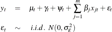 Source: [http://support.sas.com/documentation/cdl/en/etsug/66840/HTML/default/viewer.htm#etsug_ucm_details01.htm](http://support.sas.com/documentation/cdl/en/etsug/66840/HTML/default/viewer.htm#etsug_ucm_details01.htm)
# Predicting closing price of Google'
train_sample = google["Close"].diff().iloc[1:].values
model = sm.tsa.UnobservedComponents(train_sample,'local level')
result = model.fit(maxiter=1000,disp=False)
print(result.summary())
predicted_result = result.predict(start=0, end=500)
result.plot_diagnostics()
# calculating error
rmse = math.sqrt(mean_squared_error(train_sample[1:502], predicted_result))
print("The root mean squared error is {}.".format(rmse))
Unobserved Components Results
==============================================================================
Dep. Variable: y No. Observations: 3018
Model: local level Log Likelihood -10116.511
Date: Tue, 21 May 2019 AIC 20237.023
Time: 08:12:36 BIC 20249.047
Sample: 0 HQIC 20241.346
- 3018
Covariance Type: opg
====================================================================================
coef std err z P>|z| [0.025 0.975]
------------------------------------------------------------------------------------
sigma2.irregular 47.7219 0.384 124.248 0.000 46.969 48.475
sigma2.level 5.033e-05 0.000 0.458 0.647 -0.000 0.000
===================================================================================
Ljung-Box (Q): 82.72 Jarque-Bera (JB): 48879.50
Prob(Q): 0.00 Prob(JB): 0.00
Heteroskedasticity (H): 3.36 Skew: 1.11
Prob(H) (two-sided): 0.00 Kurtosis: 22.59
===================================================================================
Warnings:
[1] Covariance matrix calculated using the outer product of gradients (complex-step).
The root mean squared error is 4.412418985322874.

plt.plot(train_sample[1:502],color='red')
plt.plot(predicted_result,color='blue')
plt.legend(['Actual','Predicted'])
plt.title('Google Closing prices')
plt.show()

4.6.3 Dynamic Factor models
이 부분은 이해가 잘 되지 않아 번역하지 않았습니다. 국내 자료도 거의 없어 이해가 어렵네요. :-( 또한 원본 커널의 코드가 에러가 나서 코드는 생략했습니다.
Dynamic-factor models are flexible models for multivariate time series in which the observed endogenous variables are linear functions of exogenous covariates and unobserved factors, which have a vector autoregressive structure. The unobserved factors may also be a function of exogenous covariates. The disturbances in the equations for the dependent variables may be autocorrelated.
더 많은 회귀 모델을 추가할 예정입니다, 하지만 경험상 시계열 예측에 가장 적합한 모델은 LSTM 기반의 RNN 모델입니다. 이를 위해 더 상세한 튜토리얼을 준비했고, 링크는 아래와 같습니다.
References and influences(These have more in-depth content and explanations):
- Manipulating Time Series Data in Python
- Introduction to Time Series Analysis in Python
- Visualizing Time Series Data in Python
- VAR models and LSTM
- State space models
Stay tuned for more! And don't forget to upvote and comment.