Office Hours session 2
Starter code (copy from here: http://bit.ly/complex-pipeline)
import pandas as pd
from sklearn.impute import SimpleImputer
from sklearn.preprocessing import OneHotEncoder
from sklearn.feature_extraction.text import CountVectorizer
from sklearn.linear_model import LogisticRegression
from sklearn.compose import make_column_transformer
from sklearn.pipeline import make_pipeline
cols = ['Parch', 'Fare', 'Embarked', 'Sex', 'Name', 'Age']
df = pd.read_csv('http://bit.ly/kaggletrain')
X = df[cols]
y = df['Survived']
df_new = pd.read_csv('http://bit.ly/kaggletest')
X_new = df_new[cols]
imp_constant = SimpleImputer(strategy='constant', fill_value='missing')
ohe = OneHotEncoder()
imp_ohe = make_pipeline(imp_constant, ohe)
vect = CountVectorizer()
imp = SimpleImputer()
ct = make_column_transformer(
    (imp_ohe, ['Embarked', 'Sex']),
    (vect, 'Name'),
    (imp, ['Age', 'Fare']),
    remainder='passthrough')
logreg = LogisticRegression(solver='liblinear', random_state=1)
pipe = make_pipeline(ct, logreg)
pipe.fit(X, y)
pipe.predict(X_new)
array([0, 1, 0, 0, 1, 0, 1, 0, 1, 0, 0, 0, 1, 0, 1, 1, 0, 0, 0, 1, 0, 1,
       1, 0, 1, 0, 1, 0, 0, 0, 0, 0, 1, 1, 0, 0, 1, 1, 0, 0, 0, 0, 0, 1,
       1, 0, 0, 0, 1, 1, 0, 0, 1, 1, 0, 0, 0, 0, 0, 1, 0, 0, 0, 1, 1, 1,
       1, 0, 0, 1, 1, 0, 1, 0, 1, 1, 0, 1, 0, 1, 0, 1, 0, 0, 0, 0, 1, 1,
       1, 1, 1, 0, 1, 0, 0, 0, 1, 0, 1, 0, 1, 0, 0, 0, 1, 0, 0, 0, 0, 0,
       0, 1, 1, 1, 1, 0, 0, 1, 0, 1, 1, 0, 1, 0, 0, 1, 0, 1, 0, 0, 0, 0,
       0, 0, 0, 0, 0, 0, 1, 0, 0, 1, 0, 0, 0, 0, 0, 0, 0, 0, 1, 0, 0, 0,
       1, 0, 1, 1, 0, 1, 1, 1, 1, 0, 0, 1, 0, 0, 1, 1, 0, 0, 0, 0, 0, 1,
       1, 0, 1, 1, 0, 0, 1, 0, 1, 0, 1, 0, 0, 0, 0, 0, 0, 0, 1, 0, 1, 1,
       0, 1, 1, 0, 1, 1, 0, 0, 1, 0, 1, 0, 0, 0, 0, 1, 0, 0, 1, 0, 1, 0,
       1, 0, 1, 0, 1, 1, 0, 1, 0, 0, 0, 1, 0, 0, 0, 0, 0, 0, 1, 1, 1, 1,
       1, 0, 0, 0, 1, 0, 1, 1, 0, 0, 1, 0, 0, 0, 0, 0, 1, 0, 0, 0, 1, 1,
       0, 0, 0, 0, 1, 0, 0, 0, 1, 1, 0, 1, 0, 0, 0, 0, 1, 0, 1, 1, 1, 0,
       0, 0, 0, 0, 0, 1, 0, 0, 0, 0, 1, 0, 0, 0, 0, 0, 0, 0, 1, 1, 0, 1,
       0, 1, 0, 0, 0, 1, 1, 1, 1, 0, 0, 0, 0, 0, 0, 0, 1, 0, 1, 0, 0, 0,
       1, 0, 0, 1, 0, 0, 0, 0, 0, 1, 0, 0, 0, 1, 0, 1, 0, 1, 0, 1, 1, 0,
       0, 0, 1, 0, 1, 0, 0, 1, 0, 1, 1, 0, 1, 0, 0, 1, 1, 0, 0, 1, 0, 0,
       1, 1, 1, 0, 0, 1, 0, 0, 1, 1, 0, 1, 0, 0, 0, 0, 0, 1, 1, 0, 0, 1,
       0, 1, 0, 0, 1, 0, 1, 0, 0, 0, 0, 1, 1, 1, 1, 1, 1, 0, 1, 0, 0, 1])
K: Why did you create the imp_ohe pipeline? Why didn't you instead add imp_constant to the ColumnTransformer?
Here's a reminder of what imp_ohe contains:
imp_ohe = make_pipeline(imp_constant, ohe)
Here's how I used it in the ColumnTransformer:
ct = make_column_transformer(
    (imp_ohe, ['Embarked', 'Sex']),
    (vect, 'Name'),
    (imp, ['Age', 'Fare']),
    remainder='passthrough')
Many people suggested that I use something like this instead (which will not work):
ct_suggestion = make_column_transformer(
    (imp_constant, ['Embarked', 'Sex']),
    (ohe, ['Embarked', 'Sex']),
    (vect, 'Name'),
    (imp, ['Age', 'Fare']),
    remainder='passthrough')
I'll create the 10 row dataset to help me explain why:
df_tiny = df.head(10).copy()
df_tiny
| PassengerId | Survived | Pclass | Name | Sex | Age | SibSp | Parch | Ticket | Fare | Cabin | Embarked | |
|---|---|---|---|---|---|---|---|---|---|---|---|---|
| 0 | 1 | 0 | 3 | Braund, Mr. Owen Harris | male | 22.0 | 1 | 0 | A/5 21171 | 7.2500 | NaN | S |
| 1 | 2 | 1 | 1 | Cumings, Mrs. John Bradley (Florence Briggs Th... | female | 38.0 | 1 | 0 | PC 17599 | 71.2833 | C85 | C |
| 2 | 3 | 1 | 3 | Heikkinen, Miss. Laina | female | 26.0 | 0 | 0 | STON/O2. 3101282 | 7.9250 | NaN | S |
| 3 | 4 | 1 | 1 | Futrelle, Mrs. Jacques Heath (Lily May Peel) | female | 35.0 | 1 | 0 | 113803 | 53.1000 | C123 | S |
| 4 | 5 | 0 | 3 | Allen, Mr. William Henry | male | 35.0 | 0 | 0 | 373450 | 8.0500 | NaN | S |
| 5 | 6 | 0 | 3 | Moran, Mr. James | male | NaN | 0 | 0 | 330877 | 8.4583 | NaN | Q |
| 6 | 7 | 0 | 1 | McCarthy, Mr. Timothy J | male | 54.0 | 0 | 0 | 17463 | 51.8625 | E46 | S |
| 7 | 8 | 0 | 3 | Palsson, Master. Gosta Leonard | male | 2.0 | 3 | 1 | 349909 | 21.0750 | NaN | S |
| 8 | 9 | 1 | 3 | Johnson, Mrs. Oscar W (Elisabeth Vilhelmina Berg) | female | 27.0 | 0 | 2 | 347742 | 11.1333 | NaN | S |
| 9 | 10 | 1 | 2 | Nasser, Mrs. Nicholas (Adele Achem) | female | 14.0 | 1 | 0 | 237736 | 30.0708 | NaN | C |
X_tiny = df_tiny[cols]
X_tiny
| Parch | Fare | Embarked | Sex | Name | Age | |
|---|---|---|---|---|---|---|
| 0 | 0 | 7.2500 | S | male | Braund, Mr. Owen Harris | 22.0 |
| 1 | 0 | 71.2833 | C | female | Cumings, Mrs. John Bradley (Florence Briggs Th... | 38.0 |
| 2 | 0 | 7.9250 | S | female | Heikkinen, Miss. Laina | 26.0 |
| 3 | 0 | 53.1000 | S | female | Futrelle, Mrs. Jacques Heath (Lily May Peel) | 35.0 |
| 4 | 0 | 8.0500 | S | male | Allen, Mr. William Henry | 35.0 |
| 5 | 0 | 8.4583 | Q | male | Moran, Mr. James | NaN |
| 6 | 0 | 51.8625 | S | male | McCarthy, Mr. Timothy J | 54.0 |
| 7 | 1 | 21.0750 | S | male | Palsson, Master. Gosta Leonard | 2.0 |
| 8 | 2 | 11.1333 | S | female | Johnson, Mrs. Oscar W (Elisabeth Vilhelmina Berg) | 27.0 |
| 9 | 0 | 30.0708 | C | female | Nasser, Mrs. Nicholas (Adele Achem) | 14.0 |
Here's a smaller ColumnTransformer that uses imp_ohe, but only on "Embarked":
- There are no missing values, so the first step of the imp_ohe Pipeline passes it along to the second step
- The second step of the imp_ohe Pipeline does the one-hot encoding and outputs three columns
- This is exactly what we want
make_column_transformer(
    (imp_ohe, ['Embarked']),
    remainder='drop').fit_transform(X_tiny)
array([[0., 0., 1.],
       [1., 0., 0.],
       [0., 0., 1.],
       [0., 0., 1.],
       [0., 0., 1.],
       [0., 1., 0.],
       [0., 0., 1.],
       [0., 0., 1.],
       [0., 0., 1.],
       [1., 0., 0.]])
Try splitting imp_ohe into two separate transformers:
- imp_constant does the imputation, and ohe does the one-hot encoding
- The results get stacked side-by-side, which is not what we want
make_column_transformer(
    (imp_constant, ['Embarked']),
    (ohe, ['Embarked']),
    remainder='drop').fit_transform(X_tiny)
array([['S', 0.0, 0.0, 1.0],
       ['C', 1.0, 0.0, 0.0],
       ['S', 0.0, 0.0, 1.0],
       ['S', 0.0, 0.0, 1.0],
       ['S', 0.0, 0.0, 1.0],
       ['Q', 0.0, 1.0, 0.0],
       ['S', 0.0, 0.0, 1.0],
       ['S', 0.0, 0.0, 1.0],
       ['S', 0.0, 0.0, 1.0],
       ['C', 1.0, 0.0, 0.0]], dtype=object)
Try reversing the order of the transformers:
- All this does is change the order of the output columns, which is still not what we want
make_column_transformer(
    (ohe, ['Embarked']),
    (imp_constant, ['Embarked']),
    remainder='drop').fit_transform(X_tiny)
array([[0.0, 0.0, 1.0, 'S'],
       [1.0, 0.0, 0.0, 'C'],
       [0.0, 0.0, 1.0, 'S'],
       [0.0, 0.0, 1.0, 'S'],
       [0.0, 0.0, 1.0, 'S'],
       [0.0, 1.0, 0.0, 'Q'],
       [0.0, 0.0, 1.0, 'S'],
       [0.0, 0.0, 1.0, 'S'],
       [0.0, 0.0, 1.0, 'S'],
       [1.0, 0.0, 0.0, 'C']], dtype=object)
Key ideas:
- Pipeline operates sequentially
- It has steps: the output of step 1 is the input to step 2
- This applies to our larger Pipeline (pipe) and our smaller Pipeline (imp_ohe)
- ColumnTransformer operates in parallel
- It does not have steps: data does not flow from one transformer to the next
- It splits up the columns, transforms them independently, and combines the results side-by-side
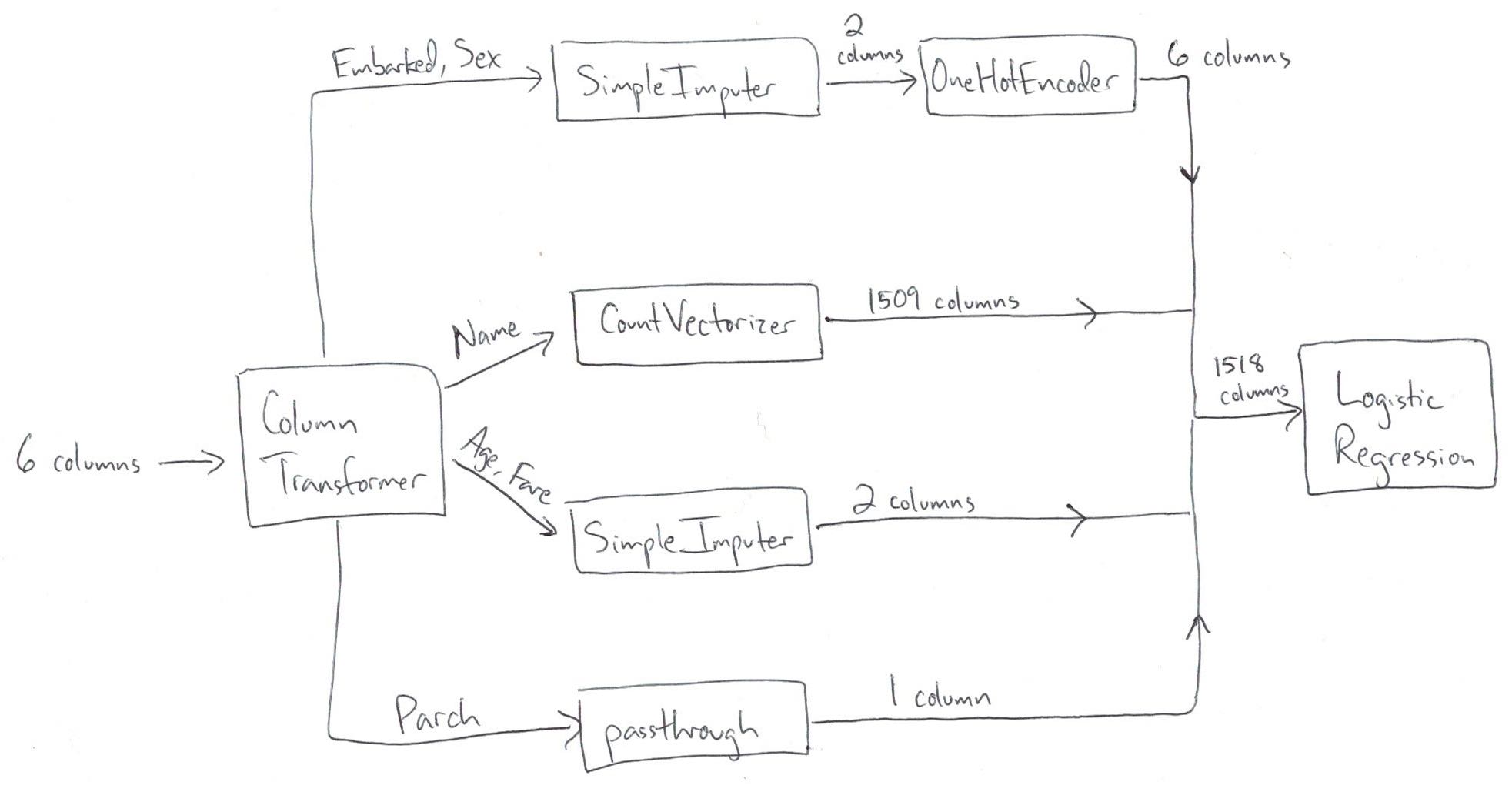
Take one more look at the correct ColumnTransformer (which matches the diagram above):
ct = make_column_transformer(
    (imp_ohe, ['Embarked', 'Sex']),
    (vect, 'Name'),
    (imp, ['Age', 'Fare']),
    remainder='passthrough')
ct.fit_transform(X)
<891x1518 sparse matrix of type '<class 'numpy.float64'>'
	with 7328 stored elements in Compressed Sparse Row format>
Compare that to the ColumnTransformer many people were suggesting:
- The first transformer (imp_constant) operates completely independently of the second transformer (ohe)
- imp_constant doesn't pass transformed data down to the second transformer
ct_suggestion = make_column_transformer(
    (imp_constant, ['Embarked', 'Sex']),
    (ohe, ['Embarked', 'Sex']),
    (vect, 'Name'),
    (imp, ['Age', 'Fare']),
    remainder='passthrough')
It will error during fit_transform because the ohe transformer doesn't know how to handle missing values:
# ct_suggestion.fit_transform(X)
Justin: What's the cost versus the benefit of adding so many columns for Name?
Cross-validate our pipeline:
- Use IPython's "time" magic function to time how long the operation takes
- This accuracy score is our baseline score
- 1509 of the 1518 features were created by the "Name" column
from sklearn.model_selection import cross_val_score
%time cross_val_score(pipe, X, y, cv=5, scoring='accuracy').mean()
CPU times: user 112 ms, sys: 2.32 ms, total: 114 ms
Wall time: 114 ms
0.8114619295712762
Remove "Name" from the ColumnTransformer:
- Using this notation is an easy way to drop some columns ("Name") and passthrough other columns ("Parch")
- This results in only 9 features
ct_no_name = make_column_transformer(
    (imp_ohe, ['Embarked', 'Sex']),
    ('drop', 'Name'),
    (imp, ['Age', 'Fare']),
    remainder='passthrough')
Cross-validate the pipeline that doesn't include "Name":
no_name = make_pipeline(ct_no_name, logreg)
%time cross_val_score(no_name, X, y, cv=5, scoring='accuracy').mean()
CPU times: user 65.8 ms, sys: 1.23 ms, total: 67 ms
Wall time: 68.1 ms
0.7833908731404181
Create a pipeline that only includes "Name" and cross-validate it:
- Since we're only using one column, there's no need for a ColumnTransformer
- Pass the "Name" Series (rather than the entire X) to cross_val_score
- This results in 1509 features
only_name = make_pipeline(vect, logreg)
%time cross_val_score(only_name, X['Name'], y, cv=5, scoring='accuracy').mean()
CPU times: user 44 ms, sys: 1.4 ms, total: 45.4 ms
Wall time: 45.6 ms
0.7945954428472788
What were the results?
- The best results came from using all of our features
- only_name had a slightly higher accuracy than no_name
- only_name ran slightly faster than no_name (probably because there's overhead from the ColumnTransformer)
What are the benefits of including "Name"?
- Better accuracy, which tells us that the "Name" column contains more signal than noise (with respect to the target)
What are the costs of including "Name"?
- Less interpretability, since it's impractical to examine the coefficients of 1518 features
Other thoughts:
- Including "Name" in this model is not resulting in overfitting, since it's increasing the cross-validated accuracy
- As demonstrated in this example, having more features (1518) than observations (891) does not automatically result in overfitting
- It's possible that including "Name" would make some models worse, but you shouldn't assume that without trying it
Anton: What's the target accuracy that you are trying to reach?
- For most real problems, it's impossible to know how accurate your model could be if you did enough tuning and tried enough models
- It's also impossible to know how accurate your model could be if you got more observations or more features
- Thus in most cases, you don't have a target accuracy, instead you just stop once you run out of time or money or ideas
- The main exception is if you are working on a well-studied research problem, because in that case there may be a state-of-the-art benchmark that everyone is trying to surpass
Motasem: When using cross_val_score, is the imputation value calculated separately for each fold?
Here's a reminder of what our ColumnTransformer and Pipeline look like:
ct = make_column_transformer(
    (imp_ohe, ['Embarked', 'Sex']),
    (vect, 'Name'),
    (imp, ['Age', 'Fare']),
    remainder='passthrough')
pipe = make_pipeline(ct, logreg)
Here's a reminder of how we cross-validate the Pipeline:
cross_val_score(pipe, X, y, cv=5, scoring='accuracy').mean()
0.8114619295712762
What happens "under the hood" when we run cross_val_score?
- Step 1: cross_val_score splits the data, such that 80% is set aside for training and the remaining 20% is set aside for testing
- Step 2: pipe.fit is run on the training portion, which means that the transformations are performed on the training portion and the transformed data is used to fit the model
- Step 3: pipe.predict is run on the testing portion, which means that the transformations are applied to the testing portion and the transformed data is passed to the model for predictions
- Step 4: The accuracy of the predictions is calculated
- Steps 1 through 4 are repeated 4 more times, and each time a different 20% is set aside as the testing portion
The key point is that cross_val_score does the transformations (steps 2 and 3) after splitting the data (step 1):
- Thus, the imputation values for "Age" and "Fare" are calculated 5 different times
- Each time, these values are calculated using the training portion, and applied to both the training and testing portions
- This is done specifically to avoid data leakage, which is when you inadvertently include knowledge from the testing data when training a model
Anusha: Why would missing value imputation in pandas lead to data leakage?
- Your model evaluation procedure (cross-validation in this case) is supposed to simulate the future, so that you can accurately estimate right now how well your model will perform on new data
- If you impute missing values on your whole dataset in pandas and then pass your dataset to scikit-learn, your model evaluation procedure will no longer be an accurate simulation of reality
- This is because the imputation values are based on your entire dataset, rather than just the training portion of your dataset
- Keep in mind that the "training portion" will change 5 times during 5-fold cross-validation, thus it's impractical to avoid data leakage if you use pandas for imputation
Hause: Regarding cross_val_score, what algorithm does scikit-learn use to split the data into different folds? Can you examine the data used in each fold?
When using cross_val_score, I've been passing an integer that specifies the number of folds:
cross_val_score(pipe, X, y, cv=5, scoring='accuracy')
array([0.79888268, 0.8258427 , 0.80337079, 0.78651685, 0.84269663])
Here's what happens "under the hood" when you specify 5 folds for a classification problem:
from sklearn.model_selection import StratifiedKFold
kf = StratifiedKFold(5)
cross_val_score(pipe, X, y, cv=kf, scoring='accuracy')
array([0.79888268, 0.8258427 , 0.80337079, 0.78651685, 0.84269663])
StratifiedKFold is a cross-validation splitter, meaning that its role is to split datasets:
- You pass the splitter to cross_val_score instead of an integer
- "Stratified" means that it uses stratified sampling to ensure that the class frequencies are approximately equal in each split
- Example: 38% of the y values are 1 (which means survived), so every time it splits, it ensures that about 38% of the training portion is survived passengers and about 38% of the testing portion is survived passengers
You can examine the data used in each fold. Here are the training and testing indices used by the first split:
list(kf.split(X, y))[0]
(array([168, 169, 170, 171, 173, 174, 175, 176, 177, 178, 179, 180, 181,
        182, 185, 188, 189, 191, 196, 197, 199, 200, 201, 202, 203, 204,
        205, 206, 207, 208, 209, 210, 211, 212, 213, 214, 215, 216, 217,
        218, 219, 220, 221, 222, 223, 224, 225, 226, 227, 228, 229, 230,
        231, 232, 233, 234, 235, 236, 237, 238, 239, 240, 241, 242, 243,
        244, 245, 246, 247, 248, 249, 250, 251, 252, 253, 254, 255, 256,
        257, 258, 259, 260, 261, 262, 263, 264, 265, 266, 267, 268, 269,
        270, 271, 272, 273, 274, 275, 276, 277, 278, 279, 280, 281, 282,
        283, 284, 285, 286, 287, 288, 289, 290, 291, 292, 293, 294, 295,
        296, 297, 298, 299, 300, 301, 302, 303, 304, 305, 306, 307, 308,
        309, 310, 311, 312, 313, 314, 315, 316, 317, 318, 319, 320, 321,
        322, 323, 324, 325, 326, 327, 328, 329, 330, 331, 332, 333, 334,
        335, 336, 337, 338, 339, 340, 341, 342, 343, 344, 345, 346, 347,
        348, 349, 350, 351, 352, 353, 354, 355, 356, 357, 358, 359, 360,
        361, 362, 363, 364, 365, 366, 367, 368, 369, 370, 371, 372, 373,
        374, 375, 376, 377, 378, 379, 380, 381, 382, 383, 384, 385, 386,
        387, 388, 389, 390, 391, 392, 393, 394, 395, 396, 397, 398, 399,
        400, 401, 402, 403, 404, 405, 406, 407, 408, 409, 410, 411, 412,
        413, 414, 415, 416, 417, 418, 419, 420, 421, 422, 423, 424, 425,
        426, 427, 428, 429, 430, 431, 432, 433, 434, 435, 436, 437, 438,
        439, 440, 441, 442, 443, 444, 445, 446, 447, 448, 449, 450, 451,
        452, 453, 454, 455, 456, 457, 458, 459, 460, 461, 462, 463, 464,
        465, 466, 467, 468, 469, 470, 471, 472, 473, 474, 475, 476, 477,
        478, 479, 480, 481, 482, 483, 484, 485, 486, 487, 488, 489, 490,
        491, 492, 493, 494, 495, 496, 497, 498, 499, 500, 501, 502, 503,
        504, 505, 506, 507, 508, 509, 510, 511, 512, 513, 514, 515, 516,
        517, 518, 519, 520, 521, 522, 523, 524, 525, 526, 527, 528, 529,
        530, 531, 532, 533, 534, 535, 536, 537, 538, 539, 540, 541, 542,
        543, 544, 545, 546, 547, 548, 549, 550, 551, 552, 553, 554, 555,
        556, 557, 558, 559, 560, 561, 562, 563, 564, 565, 566, 567, 568,
        569, 570, 571, 572, 573, 574, 575, 576, 577, 578, 579, 580, 581,
        582, 583, 584, 585, 586, 587, 588, 589, 590, 591, 592, 593, 594,
        595, 596, 597, 598, 599, 600, 601, 602, 603, 604, 605, 606, 607,
        608, 609, 610, 611, 612, 613, 614, 615, 616, 617, 618, 619, 620,
        621, 622, 623, 624, 625, 626, 627, 628, 629, 630, 631, 632, 633,
        634, 635, 636, 637, 638, 639, 640, 641, 642, 643, 644, 645, 646,
        647, 648, 649, 650, 651, 652, 653, 654, 655, 656, 657, 658, 659,
        660, 661, 662, 663, 664, 665, 666, 667, 668, 669, 670, 671, 672,
        673, 674, 675, 676, 677, 678, 679, 680, 681, 682, 683, 684, 685,
        686, 687, 688, 689, 690, 691, 692, 693, 694, 695, 696, 697, 698,
        699, 700, 701, 702, 703, 704, 705, 706, 707, 708, 709, 710, 711,
        712, 713, 714, 715, 716, 717, 718, 719, 720, 721, 722, 723, 724,
        725, 726, 727, 728, 729, 730, 731, 732, 733, 734, 735, 736, 737,
        738, 739, 740, 741, 742, 743, 744, 745, 746, 747, 748, 749, 750,
        751, 752, 753, 754, 755, 756, 757, 758, 759, 760, 761, 762, 763,
        764, 765, 766, 767, 768, 769, 770, 771, 772, 773, 774, 775, 776,
        777, 778, 779, 780, 781, 782, 783, 784, 785, 786, 787, 788, 789,
        790, 791, 792, 793, 794, 795, 796, 797, 798, 799, 800, 801, 802,
        803, 804, 805, 806, 807, 808, 809, 810, 811, 812, 813, 814, 815,
        816, 817, 818, 819, 820, 821, 822, 823, 824, 825, 826, 827, 828,
        829, 830, 831, 832, 833, 834, 835, 836, 837, 838, 839, 840, 841,
        842, 843, 844, 845, 846, 847, 848, 849, 850, 851, 852, 853, 854,
        855, 856, 857, 858, 859, 860, 861, 862, 863, 864, 865, 866, 867,
        868, 869, 870, 871, 872, 873, 874, 875, 876, 877, 878, 879, 880,
        881, 882, 883, 884, 885, 886, 887, 888, 889, 890]),
 array([  0,   1,   2,   3,   4,   5,   6,   7,   8,   9,  10,  11,  12,
         13,  14,  15,  16,  17,  18,  19,  20,  21,  22,  23,  24,  25,
         26,  27,  28,  29,  30,  31,  32,  33,  34,  35,  36,  37,  38,
         39,  40,  41,  42,  43,  44,  45,  46,  47,  48,  49,  50,  51,
         52,  53,  54,  55,  56,  57,  58,  59,  60,  61,  62,  63,  64,
         65,  66,  67,  68,  69,  70,  71,  72,  73,  74,  75,  76,  77,
         78,  79,  80,  81,  82,  83,  84,  85,  86,  87,  88,  89,  90,
         91,  92,  93,  94,  95,  96,  97,  98,  99, 100, 101, 102, 103,
        104, 105, 106, 107, 108, 109, 110, 111, 112, 113, 114, 115, 116,
        117, 118, 119, 120, 121, 122, 123, 124, 125, 126, 127, 128, 129,
        130, 131, 132, 133, 134, 135, 136, 137, 138, 139, 140, 141, 142,
        143, 144, 145, 146, 147, 148, 149, 150, 151, 152, 153, 154, 155,
        156, 157, 158, 159, 160, 161, 162, 163, 164, 165, 166, 167, 172,
        183, 184, 186, 187, 190, 192, 193, 194, 195, 198]))
By default, StratifiedKFold does not shuffle the rows:
- There is no randomness in this process, thus you will always get the same results every time
- This is why cross_val_score and GridSearchCV don't have a random_state parameter
If the order of your rows is not arbitrary, then you can (and should) shuffle the rows by modifying the splitter:
kf = StratifiedKFold(5, shuffle=True, random_state=0)
Leona: Would you recommend using a validation set when tuning the model's hyperparameters?
When we use grid search, we're choosing hyperparameters that maximize the cross-validation score on this dataset:
- Thus, we're using the same data to do two separate jobs: tune the model hyperparameters and estimate its future performance
- This biases the model to this dataset and can result in overly optimistic scores
If you want a more realistic performance estimate and you have enough data to spare:
- Split the training data into two sets: the first set is passed to grid search, and second set is used to evaluate the best model chosen by grid search
- The score on the second set is a more realistic estimate of model performance because the model wasn't tuned to that set
If you want a more realistic performance estimate and you don't have enough data to spare:
- Use nested cross-validation, which has an outer loop and an inner loop:
- Inner loop does the hyperparameter tuning using grid search
- Outer loop estimates model performance using cross-validation
Bottom line:
- If you want the most realistic estimate of a model's performance, then you have to add additional complexity to your process
- If you only care about choosing the best hyperparameters, then you don't need to add this complexity
Recommended resources:
JV: What is the difference between FeatureUnion and ColumnTransformer?
As a reminder, you can add a "missing indicator" to SimpleImputer (new in version 0.21):
SimpleImputer(add_indicator=True).fit_transform(X_tiny[['Age']])
array([[22.        ,  0.        ],
       [38.        ,  0.        ],
       [26.        ,  0.        ],
       [35.        ,  0.        ],
       [35.        ,  0.        ],
       [28.11111111,  1.        ],
       [54.        ,  0.        ],
       [ 2.        ,  0.        ],
       [27.        ,  0.        ],
       [14.        ,  0.        ]])
How could we create the same output without using the "add_indicator" parameter?
We can create the left column using the SimpleImputer:
imp.fit_transform(X_tiny[['Age']])
array([[22.        ],
       [38.        ],
       [26.        ],
       [35.        ],
       [35.        ],
       [28.11111111],
       [54.        ],
       [ 2.        ],
       [27.        ],
       [14.        ]])
We can create the right column using the MissingIndicator class:
- It outputs False and True instead of 0 and 1, but otherwise the results are the same
- This is available in version 0.20
from sklearn.impute import MissingIndicator
indicator = MissingIndicator()
indicator.fit_transform(X_tiny[['Age']])
array([[False],
       [False],
       [False],
       [False],
       [False],
       [ True],
       [False],
       [False],
       [False],
       [False]])
We can use FeatureUnion to stack these two columns side-by-side:
- Use make_union to create a FeatureUnion of SimpleImputer and MissingIndicator
- False and True are converted to 0 and 1 when put in a numeric array
from sklearn.pipeline import make_union
imp_indicator = make_union(imp, indicator)
imp_indicator.fit_transform(X_tiny[['Age']])
array([[22.        ,  0.        ],
       [38.        ,  0.        ],
       [26.        ,  0.        ],
       [35.        ,  0.        ],
       [35.        ,  0.        ],
       [28.11111111,  1.        ],
       [54.        ,  0.        ],
       [ 2.        ,  0.        ],
       [27.        ,  0.        ],
       [14.        ,  0.        ]])
Comparing FeatureUnion and ColumnTransformer:
- FeatureUnion applies multiple transformations to a single input column and stacks the results side-by-side
- ColumnTransformer applies a different transformation to each input column and stacks the results side-by-side
Thus we could include our FeatureUnion in a ColumnTransformer:
make_column_transformer(
    (imp_indicator, ['Age']),
    remainder='drop').fit_transform(X_tiny)
array([[22.        ,  0.        ],
       [38.        ,  0.        ],
       [26.        ,  0.        ],
       [35.        ,  0.        ],
       [35.        ,  0.        ],
       [28.11111111,  1.        ],
       [54.        ,  0.        ],
       [ 2.        ,  0.        ],
       [27.        ,  0.        ],
       [14.        ,  0.        ]])
Or we could achieve the same results without the FeatureUnion, by passing the "Age" column to the ColumnTransformer twice:
make_column_transformer(
    (imp, ['Age']),
    (indicator, ['Age']),
    remainder='drop').fit_transform(X_tiny)
array([[22.        ,  0.        ],
       [38.        ,  0.        ],
       [26.        ,  0.        ],
       [35.        ,  0.        ],
       [35.        ,  0.        ],
       [28.11111111,  1.        ],
       [54.        ,  0.        ],
       [ 2.        ,  0.        ],
       [27.        ,  0.        ],
       [14.        ,  0.        ]])
Conclusion:
- In both FeatureUnion and ColumnTransformer, data does not flow from one transformer to the next
- Instead, the transformers are applied independently (in parallel)
- This is different from a Pipeline, in which data does flow from one step to the next
- FeatureUnion was a precursor to ColumnTransformer
- FeatureUnion is far less useful now that ColumnTransformer exists
Gloria: Can you talk about the other two imputers in scikit-learn?
IterativeImputer (new in version 0.21) is experimental, meaning the API and predictions may change:
from sklearn.experimental import enable_iterative_imputer
from sklearn.impute import IterativeImputer
Pass it "Parch" (no missing values), "Fare" (no missing values), and "Age" (1 missing value):
imp_iterative = IterativeImputer()
imp_iterative.fit_transform(X_tiny[['Parch', 'Fare', 'Age']])
array([[ 0.        ,  7.25      , 22.        ],
       [ 0.        , 71.2833    , 38.        ],
       [ 0.        ,  7.925     , 26.        ],
       [ 0.        , 53.1       , 35.        ],
       [ 0.        ,  8.05      , 35.        ],
       [ 0.        ,  8.4583    , 24.23702669],
       [ 0.        , 51.8625    , 54.        ],
       [ 1.        , 21.075     ,  2.        ],
       [ 2.        , 11.1333    , 27.        ],
       [ 0.        , 30.0708    , 14.        ]])
How it works:
- For the 9 rows in which "Age" was not missing:
- scikit-learn trains a regression model in which "Parch" and "Fare" are the features and "Age" is the target
- For the 1 row in which "Age" was missing:
- scikit-learn passes the "Parch" and "Fare" values to the trained model
- The model makes a prediction for the "Age" value, and that value is used for imputation
- In summary: IterativeImputer turned this into a regression problem with 2 features, 9 observations in the training set, and 1 observation in the testing set
Notes:
- Unlike SimpleImputer, you have to pass it multiple numeric columns, otherwise it can't do the regression problem
- Thus you're deciding what features to use in this regression problem
- You can pass it multiple features with missing values
- Meaning: "Parch", "Fare", and "Age" can all have missing values
- IterativeImputer will just do 3 different regression problems, and each column will have a turn being the target
- You can choose which regression model IterativeImputer uses
KNNImputer (new in version 0.22) is another option:
from sklearn.impute import KNNImputer
imp_knn = KNNImputer(n_neighbors=2)
imp_knn.fit_transform(X_tiny[['Parch', 'Fare', 'Age']])
array([[ 0.    ,  7.25  , 22.    ],
       [ 0.    , 71.2833, 38.    ],
       [ 0.    ,  7.925 , 26.    ],
       [ 0.    , 53.1   , 35.    ],
       [ 0.    ,  8.05  , 35.    ],
       [ 0.    ,  8.4583, 30.5   ],
       [ 0.    , 51.8625, 54.    ],
       [ 1.    , 21.075 ,  2.    ],
       [ 2.    , 11.1333, 27.    ],
       [ 0.    , 30.0708, 14.    ]])
How it works:
- For the 1 row in which "Age" was missing:
- Because I set n_neighbors=2, scikit-learn finds the 2 "nearest" rows to this row, which is measured by how close the "Parch" and "Fare" values are to this row
- scikit-learn averages the "Age" values for those 2 rows (26 and 35), and that value (30.5) is used as the imputation value
The intuition behind both of these imputers is that it can be useful to take other features into account when deciding what value to impute:
- Example: Maybe a high "Parch" and a low "Fare" is common for kids
- Thus if "Age" is missing for a row which has a high "Parch" and a low "Fare", then you should impute a low "Age" rather than then mean of "Age", which is what SimpleImputer would do
Elin: How would you add feature selection to our Pipeline?
It can be useful to add feature selection to your workflow:
- Model accuracy can be improved by removing irrelevant features (ones that are adding "noise", not "signal")
- We can automate this process by including it in our Pipeline
- I will demonstrate two of the many ways you can do this in scikit-learn: SelectPercentile and SelectFromModel
Cross-validate our pipeline (without any hyperparameter tuning) to generate a "baseline" accuracy:
cross_val_score(pipe, X, y, cv=5, scoring='accuracy').mean()
0.8114619295712762
SelectPercentile selects features based on statistical tests:
- You specify a statistical test
- It scores all features using that test
- It keeps a percentage (that you specify) of the best scoring features
Create a feature selection object:
- Pass it the statistical test
- We're using chi2, but other tests are available
- Pass it the percentile
- We're arbitrarily using 50 to keep 50% of the features (10 would keep 10% percent of the features)
from sklearn.feature_selection import SelectPercentile, chi2
selection = SelectPercentile(chi2, percentile=50)
Add feature selection to the Pipeline after the ColumnTransformer but before the model:
pipe_selection = make_pipeline(ct, selection, logreg)
Cross-validate the updated Pipeline, and the score has improved:
cross_val_score(pipe_selection, X, y, cv=5, scoring='accuracy').mean()
0.8193019898311469
SelectFromModel scores features using a model:
- You specify a model
- Options include logistic regression, linear SVC, or any tree-based model (including ensembles)
- It uses the coef_ or feature_importances_ attribute of that model as the score
We'll try using logistic regression for feature selection:
- Create a new instance to use for feature selection
- This is completely separate from the logistic regression model we are using to make predictions
logreg_selection = LogisticRegression(solver='liblinear', penalty='l1', random_state=1)
Create a feature selection object:
- Pass it the model we're using for selection
- Pass it the threshold
- This can be the mean or median of the scores, though you can optionally include a scaling factor (such as 1.5 times mean)
- Higher threshold means fewer features will be kept
from sklearn.feature_selection import SelectFromModel
selection = SelectFromModel(logreg_selection, threshold='mean')
Update the Pipeline to use the new feature selection object:
pipe_selection = make_pipeline(ct, selection, logreg)
Cross-validate the updated Pipeline, and the score has improved again:
cross_val_score(pipe_selection, X, y, cv=5, scoring='accuracy').mean()
0.8260121775155358
Both of these approaches should be further tuned:
- With SelectPercentile you should tune the percentile, and with SelectFromModel you should tune the threshold
- You should also tune the transformer and model hyperparameters at the same time (using GridSearchCV), because you don't know which combination will produce the best results
Khaled: How would you add feature standardization to our Pipeline?
Some (but not all) Machine Learning models benefit from feature standardization, and this is often done with StandardScaler:
from sklearn.preprocessing import StandardScaler
scaler = StandardScaler()
Here's a reminder of our existing ColumnTransformer:
ct = make_column_transformer(
    (imp_ohe, ['Embarked', 'Sex']),
    (vect, 'Name'),
    (imp, ['Age', 'Fare']),
    remainder='passthrough')
If we wanted to scale "Age" and "Fare", we could make a Pipeline of imputation and scaling:
imp_scaler = make_pipeline(imp, scaler)
Then replace imp with imp_scaler in our ColumnTransformer:
ct_scaler = make_column_transformer(
    (imp_ohe, ['Embarked', 'Sex']),
    (vect, 'Name'),
    (imp_scaler, ['Age', 'Fare']),
    remainder='passthrough')
Update the Pipeline:
pipe_scaler = make_pipeline(ct_scaler, logreg)
Cross-validated accuracy has decreased slightly:
- Don't assume that scaling is always needed
- Our particular logisitic regression solver (liblinear) is robust to unscaled data
cross_val_score(pipe_scaler, X, y, cv=5, scoring='accuracy').mean()
0.8092210156299039
An alternative way to include scaling is to scale all columns:
- StandardScaler will destroy the sparsity in a sparse matrix, so use MaxAbsScaler instead
from sklearn.preprocessing import MaxAbsScaler
scaler = MaxAbsScaler()
Update the Pipeline:
- Use the original ColumnTransformer (does not include scaling)
- MaxAbsScaler is the second step
pipe_scaler = make_pipeline(ct, scaler, logreg)
Cross-validated accuracy is basically the same as our baseline (which did not include scaling):
cross_val_score(pipe_scaler, X, y, cv=5, scoring='accuracy').mean()
0.8114556525014123
Hussain: Should we scale all features, or only the features that were originally numerical?
We tried both approaches above:
- First, I only scaled the features that were originally numerical
- Second, I scaled everything that came out of the ColumnTransformer
- MaxAbsScaler has zero effect on columns output by OneHotEncoder and only a tiny effect on columns output by CountVectorizer, so the second approach is mostly just affecting the numerical columns anyway
I suggest trying both approaches, and see which one works better:
- It's not clear to me if one approach is more theoretically sound than the other
Gaurav: How would you add outlier handling to our Pipeline?
Here are two approaches you can try:
- Use a scaler that is robust to outliers (such as RobustScaler in scikit-learn)
- You can add that to a Pipeline
- Identify and remove outliers from the dataset
- There are multiple outlier detection functions in scikit-learn
- But, scikit-learn doesn't currently support transformers that remove rows, which is what you would need in order to include outlier removal in a Pipeline
Feel free to email me if you have other suggestions for outlier handling!
Leona: How would you adapt this Pipeline to use a different model, such as a RandomForestClassifier?
All that is required is switching out the final step of the Pipeline to use a different model:
- Each model has different hyperparameters you can tune, and often scikit-learn's User Guide will suggest which ones you should tune
- You should still tune all Pipeline steps simultaneously, because different models will benefit from different data transformations and different features
DS: How can I include custom transformations for feature engineering within a Pipeline?
Here's a reminder of what's in our 10 row dataset, so that we can plan out a few custom transformations:
df_tiny
| PassengerId | Survived | Pclass | Name | Sex | Age | SibSp | Parch | Ticket | Fare | Cabin | Embarked | |
|---|---|---|---|---|---|---|---|---|---|---|---|---|
| 0 | 1 | 0 | 3 | Braund, Mr. Owen Harris | male | 22.0 | 1 | 0 | A/5 21171 | 7.2500 | NaN | S |
| 1 | 2 | 1 | 1 | Cumings, Mrs. John Bradley (Florence Briggs Th... | female | 38.0 | 1 | 0 | PC 17599 | 71.2833 | C85 | C |
| 2 | 3 | 1 | 3 | Heikkinen, Miss. Laina | female | 26.0 | 0 | 0 | STON/O2. 3101282 | 7.9250 | NaN | S |
| 3 | 4 | 1 | 1 | Futrelle, Mrs. Jacques Heath (Lily May Peel) | female | 35.0 | 1 | 0 | 113803 | 53.1000 | C123 | S |
| 4 | 5 | 0 | 3 | Allen, Mr. William Henry | male | 35.0 | 0 | 0 | 373450 | 8.0500 | NaN | S |
| 5 | 6 | 0 | 3 | Moran, Mr. James | male | NaN | 0 | 0 | 330877 | 8.4583 | NaN | Q |
| 6 | 7 | 0 | 1 | McCarthy, Mr. Timothy J | male | 54.0 | 0 | 0 | 17463 | 51.8625 | E46 | S |
| 7 | 8 | 0 | 3 | Palsson, Master. Gosta Leonard | male | 2.0 | 3 | 1 | 349909 | 21.0750 | NaN | S |
| 8 | 9 | 1 | 3 | Johnson, Mrs. Oscar W (Elisabeth Vilhelmina Berg) | female | 27.0 | 0 | 2 | 347742 | 11.1333 | NaN | S |
| 9 | 10 | 1 | 2 | Nasser, Mrs. Nicholas (Adele Achem) | female | 14.0 | 1 | 0 | 237736 | 30.0708 | NaN | C |
Let's pretend we believe that "Age" and "Fare" might be better features if we floor them (meaning round them down):
- This is not possible in scikit-learn, but it is possible using NumPy's floor function
- NumPy functions are a good choice for custom transformations, because pandas and scikit-learn both work well with NumPy
- Notice that we pass it a 2D object and it returns a 2D object
- This will turn out to be a useful characteristic for custom transformations
import numpy as np
np.floor(df_tiny[['Age', 'Fare']])
| Age | Fare | |
|---|---|---|
| 0 | 22.0 | 7.0 |
| 1 | 38.0 | 71.0 |
| 2 | 26.0 | 7.0 |
| 3 | 35.0 | 53.0 |
| 4 | 35.0 | 8.0 |
| 5 | NaN | 8.0 |
| 6 | 54.0 | 51.0 |
| 7 | 2.0 | 21.0 |
| 8 | 27.0 | 11.0 |
| 9 | 14.0 | 30.0 |
In order to do this transformation in scikit-learn, we need to convert the floor function into a scikit-learn transformer using FunctionTransformer:
from sklearn.preprocessing import FunctionTransformer
Pass the floor function to FunctionTransformer and it returns a scikit-learn transformer:
- Prior to version 0.22, you should also include the argument validate=False
get_floor = FunctionTransformer(np.floor)
Because get_floor is a transformer, you can use the fit_transform method to perform transformations:
get_floor.fit_transform(df_tiny[['Age', 'Fare']])
| Age | Fare | |
|---|---|---|
| 0 | 22.0 | 7.0 |
| 1 | 38.0 | 71.0 |
| 2 | 26.0 | 7.0 |
| 3 | 35.0 | 53.0 |
| 4 | 35.0 | 8.0 |
| 5 | NaN | 8.0 |
| 6 | 54.0 | 51.0 |
| 7 | 2.0 | 21.0 |
| 8 | 27.0 | 11.0 |
| 9 | 14.0 | 30.0 |
get_floor can be included in a ColumnTransformer:
make_column_transformer(
    (get_floor, ['Age', 'Fare']),
    remainder='drop').fit_transform(df_tiny)
array([[22.,  7.],
       [38., 71.],
       [26.,  7.],
       [35., 53.],
       [35.,  8.],
       [nan,  8.],
       [54., 51.],
       [ 2., 21.],
       [27., 11.],
       [14., 30.]])
Let's plan out a second custom transformation:
- All of the cabins start with a letter, and we believe that the letter indicates the deck they were staying on, which might be a predictive feature
df_tiny
| PassengerId | Survived | Pclass | Name | Sex | Age | SibSp | Parch | Ticket | Fare | Cabin | Embarked | |
|---|---|---|---|---|---|---|---|---|---|---|---|---|
| 0 | 1 | 0 | 3 | Braund, Mr. Owen Harris | male | 22.0 | 1 | 0 | A/5 21171 | 7.2500 | NaN | S |
| 1 | 2 | 1 | 1 | Cumings, Mrs. John Bradley (Florence Briggs Th... | female | 38.0 | 1 | 0 | PC 17599 | 71.2833 | C85 | C |
| 2 | 3 | 1 | 3 | Heikkinen, Miss. Laina | female | 26.0 | 0 | 0 | STON/O2. 3101282 | 7.9250 | NaN | S |
| 3 | 4 | 1 | 1 | Futrelle, Mrs. Jacques Heath (Lily May Peel) | female | 35.0 | 1 | 0 | 113803 | 53.1000 | C123 | S |
| 4 | 5 | 0 | 3 | Allen, Mr. William Henry | male | 35.0 | 0 | 0 | 373450 | 8.0500 | NaN | S |
| 5 | 6 | 0 | 3 | Moran, Mr. James | male | NaN | 0 | 0 | 330877 | 8.4583 | NaN | Q |
| 6 | 7 | 0 | 1 | McCarthy, Mr. Timothy J | male | 54.0 | 0 | 0 | 17463 | 51.8625 | E46 | S |
| 7 | 8 | 0 | 3 | Palsson, Master. Gosta Leonard | male | 2.0 | 3 | 1 | 349909 | 21.0750 | NaN | S |
| 8 | 9 | 1 | 3 | Johnson, Mrs. Oscar W (Elisabeth Vilhelmina Berg) | female | 27.0 | 0 | 2 | 347742 | 11.1333 | NaN | S |
| 9 | 10 | 1 | 2 | Nasser, Mrs. Nicholas (Adele Achem) | female | 14.0 | 1 | 0 | 237736 | 30.0708 | NaN | C |
Use the pandas string slice method to extract the first letter:
- Use the apply method with a lambda so that it can operate on multiple columns
- This will enable our function to accept 2D input and return 2D output
df_tiny[['Cabin']].apply(lambda x: x.str.slice(0, 1))
| Cabin | |
|---|---|
| 0 | NaN |
| 1 | C |
| 2 | NaN |
| 3 | C |
| 4 | NaN |
| 5 | NaN |
| 6 | E |
| 7 | NaN |
| 8 | NaN |
| 9 | NaN |
Convert this operation into a custom function:
- You need to ensure that your function works whether the input is a DataFrame or a NumPy array
- ColumnTransformers accept both DataFrames and NumPy arrays
- Pipeline steps output NumPy arrays, which could then become the input to this function
- Thus we convert the input to a DataFrame explicitly, which ensures that we will be able to use the pandas apply method
def first_letter(df):
    return pd.DataFrame(df).apply(lambda x: x.str.slice(0, 1))
Convert the function to a transformer:
get_first_letter = FunctionTransformer(first_letter)
Add this transformer to the ColumnTransformer:
make_column_transformer(
    (get_floor, ['Age', 'Fare']),
    (get_first_letter, ['Cabin']),
    remainder='drop').fit_transform(df_tiny)
array([[22.0, 7.0, nan],
       [38.0, 71.0, 'C'],
       [26.0, 7.0, nan],
       [35.0, 53.0, 'C'],
       [35.0, 8.0, nan],
       [nan, 8.0, nan],
       [54.0, 51.0, 'E'],
       [2.0, 21.0, nan],
       [27.0, 11.0, nan],
       [14.0, 30.0, nan]], dtype=object)
Two shape considerations to keep in mind when writing functions that will be used in a ColumnTransformer:
- Your function isn't required to accept 2D input, but it's better if it accepts 2D input
- This enables your function (once transformed) to accept multiple columns in the ColumnTransformer
- Your function is required to return 2D output in order to be used in a ColumnTransformer:
- If your function returns a pandas object, it should return a DataFrame (not a Series)
- If your function returns a 1D array, reshape it (within the function) to be a 2D array
Let's plan out a third custom transformation:
- We believe that a passenger's total number of family members aboard ("SibSp" + "Parch") is more predictive than either feature individually
df_tiny
| PassengerId | Survived | Pclass | Name | Sex | Age | SibSp | Parch | Ticket | Fare | Cabin | Embarked | |
|---|---|---|---|---|---|---|---|---|---|---|---|---|
| 0 | 1 | 0 | 3 | Braund, Mr. Owen Harris | male | 22.0 | 1 | 0 | A/5 21171 | 7.2500 | NaN | S |
| 1 | 2 | 1 | 1 | Cumings, Mrs. John Bradley (Florence Briggs Th... | female | 38.0 | 1 | 0 | PC 17599 | 71.2833 | C85 | C |
| 2 | 3 | 1 | 3 | Heikkinen, Miss. Laina | female | 26.0 | 0 | 0 | STON/O2. 3101282 | 7.9250 | NaN | S |
| 3 | 4 | 1 | 1 | Futrelle, Mrs. Jacques Heath (Lily May Peel) | female | 35.0 | 1 | 0 | 113803 | 53.1000 | C123 | S |
| 4 | 5 | 0 | 3 | Allen, Mr. William Henry | male | 35.0 | 0 | 0 | 373450 | 8.0500 | NaN | S |
| 5 | 6 | 0 | 3 | Moran, Mr. James | male | NaN | 0 | 0 | 330877 | 8.4583 | NaN | Q |
| 6 | 7 | 0 | 1 | McCarthy, Mr. Timothy J | male | 54.0 | 0 | 0 | 17463 | 51.8625 | E46 | S |
| 7 | 8 | 0 | 3 | Palsson, Master. Gosta Leonard | male | 2.0 | 3 | 1 | 349909 | 21.0750 | NaN | S |
| 8 | 9 | 1 | 3 | Johnson, Mrs. Oscar W (Elisabeth Vilhelmina Berg) | female | 27.0 | 0 | 2 | 347742 | 11.1333 | NaN | S |
| 9 | 10 | 1 | 2 | Nasser, Mrs. Nicholas (Adele Achem) | female | 14.0 | 1 | 0 | 237736 | 30.0708 | NaN | C |
Use the sum method over the columns axis:
- Notice that it outputs a 1D object
df_tiny[['SibSp', 'Parch']].sum(axis=1)
0    1
1    1
2    0
3    1
4    0
5    0
6    0
7    4
8    2
9    1
dtype: int64
Convert this operation into a custom function:
- Convert the input to a NumPy array explicitly, which ensures that we will be able to use the sum and reshape methods
- Because the sum outputs a 1D object, use reshape to convert it to a 2D object
- This notation specifies that the second dimension should be 1 and the first dimension should be inferred
def sum_cols(df):
    return np.array(df).sum(axis=1).reshape(-1, 1)
Confirm that sum_cols returns 2D output:
sum_cols(df_tiny[['SibSp', 'Parch']])
array([[1],
       [1],
       [0],
       [1],
       [0],
       [0],
       [0],
       [4],
       [2],
       [1]])
Convert the function to a transformer and add it to the ColumnTransformer:
get_sum = FunctionTransformer(sum_cols)
make_column_transformer(
    (get_floor, ['Age', 'Fare']),
    (get_first_letter, ['Cabin']),
    (get_sum, ['SibSp', 'Parch']),
    remainder='drop').fit_transform(df_tiny)
array([[22.0, 7.0, nan, 1],
       [38.0, 71.0, 'C', 1],
       [26.0, 7.0, nan, 0],
       [35.0, 53.0, 'C', 1],
       [35.0, 8.0, nan, 0],
       [nan, 8.0, nan, 0],
       [54.0, 51.0, 'E', 0],
       [2.0, 21.0, nan, 4],
       [27.0, 11.0, nan, 2],
       [14.0, 30.0, nan, 1]], dtype=object)
Let's use these custom transformers on our entire dataset!
First, add "Cabin" and "SibSp" to the list of columns:
cols = ['Parch', 'Fare', 'Embarked', 'Sex', 'Name', 'Age', 'Cabin', 'SibSp']
Update X and X_new to include these columns:
X = df[cols]
X_new = df_new[cols]
Before we can add the custom transformers to our ColumnTransformer, we need to create two new Pipelines.
First, we need to account for the fact that "Age" and "Fare" have missing values:
- Thus we create a Pipeline that does imputation before flooring
imp_floor = make_pipeline(imp, get_floor)
Second, there are multiple complications with using get_first_letter on "Cabin", which you can see by examining the value_counts of the first letter:
- It contains missing values, so imputation will be required
- Letters are strings, so one-hot encoding will be required
- Some of the categories are rare (namely G and T), which can cause problems with cross-validation:
- For a rare category, it's possible for all values of that category to show up in the same testing fold during cross-validation, which will cause an error because that category was not learned during the fit step
- Thus, you have to use the handle_unknown='ignore' argument with OneHotEncoder
X['Cabin'].str.slice(0, 1).value_counts(dropna=False)
NaN    687
C       59
B       47
D       33
E       32
A       15
F       13
G        4
T        1
Name: Cabin, dtype: int64
Create a Pipeline to get the first letter, then impute a constant value, then one-hot encode the results:
- If we had done imputation as the first step (instead of the second step), the "m" of "missing" would have been extracted by get_first_letter
ohe_ignore = OneHotEncoder(handle_unknown='ignore')
letter_imp_ohe = make_pipeline(get_first_letter, imp_constant, ohe_ignore)
Add the three custom transformations to our primary ColumnTransformer:
- Use imp_floor instead of imp on "Age" and "Fare"
- Use letter_imp_ohe on "Cabin"
- Use get_sum on "SibSp" and "Parch"
- Change remainder to "drop" since all columns are now specified in the ColumnTransformer
ct = make_column_transformer(
    (imp_ohe, ['Embarked', 'Sex']),
    (vect, 'Name'),
    (imp_floor, ['Age', 'Fare']),
    (letter_imp_ohe, ['Cabin']),
    (get_sum, ['SibSp', 'Parch']),
    remainder='drop')
Update the Pipeline, fit on X, and make predictions for X_new:
pipe = make_pipeline(ct, logreg)
pipe.fit(X, y)
pipe.predict(X_new)
array([0, 1, 0, 0, 1, 0, 1, 0, 1, 0, 0, 0, 1, 0, 1, 1, 0, 0, 0, 1, 0, 1,
       1, 0, 1, 0, 1, 0, 0, 0, 0, 0, 1, 1, 0, 0, 1, 1, 0, 0, 0, 0, 0, 1,
       1, 0, 0, 0, 1, 1, 0, 0, 1, 1, 0, 0, 0, 0, 0, 1, 0, 0, 0, 1, 1, 1,
       1, 0, 0, 1, 1, 0, 1, 1, 1, 1, 0, 1, 0, 1, 1, 0, 0, 0, 0, 0, 1, 1,
       1, 1, 1, 0, 1, 0, 0, 0, 1, 0, 1, 0, 1, 0, 0, 0, 1, 0, 0, 0, 0, 0,
       0, 1, 1, 1, 1, 0, 0, 1, 0, 1, 1, 0, 1, 0, 0, 1, 0, 1, 0, 0, 0, 0,
       0, 0, 0, 0, 0, 0, 1, 0, 0, 1, 0, 0, 0, 0, 1, 0, 0, 0, 1, 0, 0, 0,
       0, 0, 1, 1, 0, 1, 1, 1, 1, 0, 0, 1, 0, 0, 1, 1, 0, 0, 0, 0, 0, 1,
       1, 0, 1, 1, 0, 1, 1, 0, 1, 0, 1, 0, 0, 0, 0, 0, 0, 0, 1, 0, 1, 1,
       0, 1, 1, 0, 1, 1, 0, 0, 1, 0, 1, 0, 0, 0, 0, 1, 0, 0, 1, 0, 1, 0,
       1, 0, 1, 0, 1, 1, 0, 1, 0, 0, 0, 1, 0, 0, 0, 0, 0, 0, 1, 1, 1, 1,
       1, 0, 0, 0, 1, 0, 1, 1, 1, 0, 0, 0, 0, 0, 0, 0, 1, 0, 0, 0, 1, 1,
       0, 0, 0, 0, 1, 0, 0, 0, 1, 1, 0, 1, 0, 0, 0, 0, 1, 1, 1, 1, 0, 0,
       0, 0, 0, 0, 0, 1, 0, 0, 0, 0, 1, 0, 0, 0, 0, 1, 0, 0, 1, 1, 0, 1,
       0, 1, 0, 0, 0, 1, 1, 1, 1, 0, 0, 0, 0, 0, 0, 0, 1, 0, 1, 0, 0, 0,
       1, 0, 0, 1, 0, 0, 0, 0, 0, 1, 0, 0, 0, 1, 0, 1, 0, 1, 0, 1, 1, 0,
       0, 0, 1, 1, 1, 0, 0, 1, 0, 1, 1, 0, 1, 0, 0, 1, 1, 0, 0, 1, 0, 0,
       1, 1, 0, 0, 0, 1, 0, 0, 1, 1, 0, 1, 0, 0, 0, 0, 1, 1, 1, 0, 0, 1,
       0, 1, 0, 0, 1, 0, 1, 0, 1, 1, 0, 0, 1, 1, 1, 1, 1, 0, 1, 0, 0, 1])
Cross-validate the Pipeline:
- The accuracy has improved from our baseline, and could be further increased through hyperparameter tuning
cross_val_score(pipe, X, y, cv=5, scoring='accuracy').mean()
0.8271420500910175
Even though it's more work to do these custom transformations in scikit-learn, there are some considerable benefits:
- Since all of the transformations are in a Pipeline, they can all be tuned using a grid search
- It won't take any extra work to apply these same transformations to new data
- There's no possibility of data leakage
JV: How can I keep up-to-date with new features that are released in scikit-learn?
Read the what's new page for all major releases:
- Scan the entire page looking for features and enhancements that interest you
- Read the class documentation if you want to know more about a new feature
- Read the GitHub pull request if you want to know the detailed history of a feature
- Alternatively, you could just read the Release Highlights, but you will miss out on a lot
Otherwise, just watch out for tutorials that teach new scikit-learn features:
- Feel free to email me if you have suggestions for blogs that I should follow!
Hause: What books or online courses would you recommend to learn more about the theory/math behind Machine Learning? Especially resources that teach theory/math but also use scikit-learn?
- My top pick is An Introduction to Statistical Learning:
- It does an excellent job explaining Machine Learning theory
- It's available as a free PDF
- It uses R, but you can read the book without knowing any R
- Feel free to email me if you have read a similar book that uses scikit-learn instead!