Notebook

Python/Numpy tutorial - Part 1: Arrays¶

NumPy is the core module for scientific computing with Python. Its operation is mainly based on N-dimensional arrays.

Arrays are the typical data structure used for analysis in data science and statistics. Arrays in NumPy are represented by N-dimensional objects called ndarrays which allows data storage, manipulation, processing and modeling.

This first tutorial is intended to show you the basic operations and used of ndarrays using NumPy. Let's start by importing NumPy library with the following command.

In [1]:

import numpy as np

The rest of tutorial is organized as follows:

Numpy Basics
- NumPy arrays basic properties
- Array creation and initialization
- Basic operations with arrays
- Arrays indexing and element access
- Stacking and splitting arrays
- Linear Algebra operations
NumPy programming exercises
- Problem 1: Linear system solver
- Problem 2: Linear regression trough least square optimization

1. NumPy Basics¶

NumPy arrays basic properties¶

When an array is created as an instance of ndarray class of Numpy, it is possible to see some of its attributes such as the information about its structure, shape and data content.

In [2]:

arr = np.array([[1,2,3],[4,5,6]]) # Create a 2x3 array filled with integer numbers
print "arr=\n",arr,"\n"
print "'arr' has shape:", arr.shape
print "'arr' has", arr.ndim,"dimensions"
print "'arr' has",arr.size,"elements"
print "'arr' has type:",arr.dtype
print "'arr' occupies",arr.nbytes,"Bytes"

arr=
[[1 2 3]
 [4 5 6]] 

'arr' has shape: (2, 3)
'arr' has 2 dimensions
'arr' has 6 elements
'arr' has type: int64
'arr' occupies 48 Bytes

Array creation and initialization¶

You can create arrays in several ways:

Manually, using np.arra function
Using prefilled placeholder such as np.zeros, np.ones, np.eye
From sequences, using np.arange, np.linspace, np.logspace
Restructuring data sequences with np.reshape
And more...

In [3]:

a = np.array([1,2,3]) # a row vector
print "\nRow vector:\n",a
a = np.array([[1],[2],[3]]) # a column vector
print "\nColumn vector:\n",a
a = np.empty((4,4)) #4x4 without initialization
print "\n4x4 uninitialized array:\n",a
a = np.zeros((4,4,)) #4x4 with zeros
print "\n4x4 array filled with zeros:\n",a
a = np.ones((4,4)) #4x4 with ones
print "\n4x4 array filled with ones\n",a
a = np.eye(4,4) #Square identity 5x5 matrix
print "\n4x4 identity array\n",a
a = np.random.rand(4,4) #4x4 with pseudo-random values
print "\n4x4 array filled with random values\n",a
a = np.arange(16) #0-15 sequence vector
print "\na vector sequence\n",a
a = np.reshape(a,(4,4)) #resized as 4x4 matrix
print "\nnow as a 4x4 array\n",a
a = np.arange(16).reshape(4,4) #a shorter way
print "\nsame 4x4 array (but created with just one command):\n",a
a = np.linspace(1,10,19) #sequence of 19 linearly spaced values from 0 to 2pi
print "\na linspace vector:\n",a
a = np.logspace(0,10,11,base=2.0) #sequence of 11 values from 2^0 to 2^10 evenly spaced values in a logaritmic scale 
print "\na logspace vector:\n",a

Row vector:
[1 2 3]

Column vector:
[[1]
 [2]
 [3]]

4x4 uninitialized array:
[[7.13276025e+247 5.01163213e+217 5.49419094e-143 9.80058441e+252]
 [1.30304358e-142 5.02034658e+175 3.40805230e+175 9.12858936e+169]
 [1.60050307e-047 1.37015525e-071 1.11763125e+261 1.16318408e-028]
 [3.97062322e+246 1.16318408e-028 5.10872156e-066 4.03551679e+175]]

4x4 array filled with zeros:
[[0. 0. 0. 0.]
 [0. 0. 0. 0.]
 [0. 0. 0. 0.]
 [0. 0. 0. 0.]]

4x4 array filled with ones
[[1. 1. 1. 1.]
 [1. 1. 1. 1.]
 [1. 1. 1. 1.]
 [1. 1. 1. 1.]]

4x4 identity array
[[1. 0. 0. 0.]
 [0. 1. 0. 0.]
 [0. 0. 1. 0.]
 [0. 0. 0. 1.]]

4x4 array filled with random values
[[0.2198821  0.61648277 0.35095399 0.28643024]
 [0.08967578 0.40549732 0.06805227 0.59707167]
 [0.41789333 0.17279681 0.82111456 0.68495884]
 [0.6831512  0.66955439 0.31166352 0.36890697]]

a vector sequence
[ 0  1  2  3  4  5  6  7  8  9 10 11 12 13 14 15]

now as a 4x4 array
[[ 0  1  2  3]
 [ 4  5  6  7]
 [ 8  9 10 11]
 [12 13 14 15]]

same 4x4 array (but created with just one command):
[[ 0  1  2  3]
 [ 4  5  6  7]
 [ 8  9 10 11]
 [12 13 14 15]]

a linspace vector:
[ 1.   1.5  2.   2.5  3.   3.5  4.   4.5  5.   5.5  6.   6.5  7.   7.5
  8.   8.5  9.   9.5 10. ]

a logspace vector:
[1.000e+00 2.000e+00 4.000e+00 8.000e+00 1.600e+01 3.200e+01 6.400e+01
 1.280e+02 2.560e+02 5.120e+02 1.024e+03]

Basic operations with arrays¶

NumPy allows to manipulate and operate arrays structures as whole object; unlike other languages, such as C++ or Java, which are forced to access and operate arrays element-by-element using for-loops or similar programming structures.

This is similar to work with MATLAB matrices. However, NumPy operators such as +, * and /, works element-wise instead of perform linear algebra operations (as MATLAB does). Element-wise operations allows NumPy to support broadcasting, an interesting feature that allows arthmetics operations with arrays of diferent sizes. In those cases, if one of the dimensions of the smaller array is equal to one, the array is spread out along the larger array to fulfill the operation.

Additionally, array objects provide some built-in functions that allow to implement some common calculations on the array such as its mean, standard deviation, maximum, minimum, etc.

In [4]:

a = np.array([[30.0, 20.0, 10.0, 0.0],[10.0, 20.0, 30.0, 40.0]])
print "a=\n",a
b = np.array([1.0, 2.0, 3.0, 4.0])
print "b=\n",b

### Broadcast operations ###
print "\na+b=\n",a+b
print "\na/b=\n",a/b
print "\na**2=\n",a**2
print "\nexp(a)=\n",np.exp(a)

### Some built-in operations ###
print "\nmean of 'a':\n", a.mean()
print "\n'a' standard deviation:\n", a.std()
print "\n'a' maximum:\n", a.max()
print "\n'a' minimum:\n", a.min()
print "\nsum of elements in 'a':\n", a.sum()
a.sort(axis=1)
print "\n'a' sorted:\n", a

a=
[[30. 20. 10.  0.]
 [10. 20. 30. 40.]]
b=
[1. 2. 3. 4.]

a+b=
[[31. 22. 13.  4.]
 [11. 22. 33. 44.]]

a/b=
[[30.         10.          3.33333333  0.        ]
 [10.         10.         10.         10.        ]]

a**2=
[[ 900.  400.  100.    0.]
 [ 100.  400.  900. 1600.]]

exp(a)=
[[1.06864746e+13 4.85165195e+08 2.20264658e+04 1.00000000e+00]
 [2.20264658e+04 4.85165195e+08 1.06864746e+13 2.35385267e+17]]

mean of 'a':
20.0

'a' standard deviation:
12.24744871391589

'a' maximum:
40.0

'a' minimum:
0.0

sum of elements in 'a':
160.0

'a' sorted:
[[ 0. 10. 20. 30.]
 [10. 20. 30. 40.]]

Arrays indexing and element access¶

Elements in NumPy arrays can also be accessed using square brackets "[ ]". Unlike other programming languages, NumPy can access elements in normal or reverse order using indices in the following way:

a[0], a[1], a[2] allows to access $a_0, a_1, a_2$ respectively being $a_0$ the first element
a[-1], a[-2], a[-3] allows to access $a_{n-1}, a_{n-2} a_{n-3}$ respectively being $a_{n-1}$ the last element

You can also select array subsets instead of unique values. To do that, use the operator : in one or more dimensions to specify the range of values to be selected.

a[m:n] selects the subset including values between $a_m$ to $a_{n-1}$ (inclusive)
a[:] selects the whole range along one dimension

Finally, you can use a custom range of values (using another array or a sequence of values) to access specific elements into an array. You can also select those values which satisfy a condition using logical operators such as: <, > or ==

In [5]:

a = np.random.randint(0,9,size=(5,5))
print "a=\n",a

### Accessing rows ###
print "\nall elememts in 'a' second row:\n",a[1,:]
### Accessing colums ###
print "\nall elememts in 'a' third column:\n",a[:,2]
### First element ###
print "\n First element: \n",a[0,0]
### Last element ###
print "\nLast element:\n",a[-1,-1]
### 3x3 subset ###
print "\nmiddle 3x3 subset:\n",a[1:4,1:4]
### Masking ###
print "\nelements greater than 5:\n",a[a>5]

a=
[[6 3 3 1 4]
 [6 1 4 4 3]
 [4 5 2 0 8]
 [7 7 5 5 3]
 [0 0 7 6 2]]

all elememts in 'a' second row:
[6 1 4 4 3]

all elememts in 'a' third column:
[3 4 2 5 7]

 First element: 
6

Last element:
2

middle 3x3 subset:
[[1 4 4]
 [5 2 0]
 [7 5 5]]

elements greater than 5:
[6 6 8 7 7 7 6]

Stacking and splitting arrays¶

Arrays can be concatenated, horizontally or vertically, with other arrays compatible in size. You can also split one array in two, or change its shape keeping the same number of elements.

In [6]:

a = np.array([[1,3,-2,2],[-5,4,5,-1],[6,-7,0,1],[5,-9,7,1]])
print "a=\n",a
b = np.array([[1,1,1,1],[2,2,2,2],[3,3,3,3],[4,4,4,4]])
print "\nb=\n",b

print "\nConcatenate 'a','b' along rows: \n",np.hstack((a,b))
print "\nConcatenate 'a','b' along columns: \n",np.vstack((a,b))
print "\nSplit 'a' along columns: \n",np.hsplit(a,2)[0],"\nand\n",np.hsplit(a,2)[1]
print "\nSplit 'b' along rows: \n",np.vsplit(b,2)[0],"\nand\n",np.vsplit(b,2)[1]
print "\n'a' reshaped into a 8x2 array \n",a.reshape((8,2))
print "\n'b' reshaped into into 2x8 array \n",b.reshape((2,8))

a=
[[ 1  3 -2  2]
 [-5  4  5 -1]
 [ 6 -7  0  1]
 [ 5 -9  7  1]]

b=
[[1 1 1 1]
 [2 2 2 2]
 [3 3 3 3]
 [4 4 4 4]]

Concatenate 'a','b' along rows: 
[[ 1  3 -2  2  1  1  1  1]
 [-5  4  5 -1  2  2  2  2]
 [ 6 -7  0  1  3  3  3  3]
 [ 5 -9  7  1  4  4  4  4]]

Concatenate 'a','b' along columns: 
[[ 1  3 -2  2]
 [-5  4  5 -1]
 [ 6 -7  0  1]
 [ 5 -9  7  1]
 [ 1  1  1  1]
 [ 2  2  2  2]
 [ 3  3  3  3]
 [ 4  4  4  4]]

Split 'a' along columns: 
[[ 1  3]
 [-5  4]
 [ 6 -7]
 [ 5 -9]] 
and
[[-2  2]
 [ 5 -1]
 [ 0  1]
 [ 7  1]]

Split 'b' along rows: 
[[1 1 1 1]
 [2 2 2 2]] 
and
[[3 3 3 3]
 [4 4 4 4]]

'a' reshaped into a 8x2 array 
[[ 1  3]
 [-2  2]
 [-5  4]
 [ 5 -1]
 [ 6 -7]
 [ 0  1]
 [ 5 -9]
 [ 7  1]]

'b' reshaped into into 2x8 array 
[[1 1 1 1 2 2 2 2]
 [3 3 3 3 4 4 4 4]]

Linear Algebra operations¶

Common matrix operations such as addition or product can be implemented in NumPy using specific operators like + or @ with ndarrays, or using MATLAB-like operators (+,*) with a different type of NumPy object called matrix (@ operator is only available for Python >= 3.5). Complex operations such as the estimation of the determinant of a matrix, its inverse, or their eigenvalues, requires the use of specific functions included in NumPy or numpy.linalg submodule.

Here are some examples of linear algebra operations with NumPy

In [7]:

a = np.random.randint(0,9,size=(5,5)).astype('float')
print "a=\n",a
b = np.random.randint(0,9,size=(5,5)).astype('float')
print "b=\n",b

a_t = a.T
print "\na transpose\n",a_t

a_inv = np.linalg.inv(a)
print "\na inverse\n", a_inv

mat_prod = np.dot(a,b)
print "\nmatricial product (a x b) (dot function)\n", np.round(mat_prod)
mat_prod = np.asmatrix(a) * np.asmatrix(b)
print "\nmatricial product (a x b) (* operator)\n", np.round(mat_prod)

a_det = np.linalg.det(a)
print "\na determinant\n", a_det

a=
[[6. 1. 7. 7. 8.]
 [8. 2. 2. 1. 6.]
 [3. 7. 2. 1. 7.]
 [3. 7. 6. 3. 0.]
 [2. 6. 7. 3. 3.]]
b=
[[4. 1. 7. 5. 6.]
 [7. 6. 0. 5. 7.]
 [4. 7. 8. 7. 5.]
 [1. 7. 0. 0. 2.]
 [5. 8. 5. 7. 5.]]

a transpose
[[6. 8. 3. 3. 2.]
 [1. 2. 7. 7. 6.]
 [7. 2. 2. 6. 7.]
 [7. 1. 1. 3. 3.]
 [8. 6. 7. 0. 3.]]

a inverse
[[-0.01490093  0.14327821 -0.06107745  0.11167513 -0.10430653]
 [-0.01817586 -0.05600131  0.12330113  0.14720812 -0.12723105]
 [-0.08220075  0.09808417 -0.17209759 -0.20812183  0.42459473]
 [ 0.22171279 -0.20877681  0.11757     0.29441624 -0.44801048]
 [ 0.01637465 -0.00360242  0.07810709 -0.17766497  0.11462256]]

matricial product (a x b) (dot function)
[[106. 174. 138. 140. 132.]
 [ 85.  89. 102. 106. 104.]
 [105. 122.  72. 113. 114.]
 [ 88. 108.  69.  92. 103.]
 [ 96. 132.  85. 110. 110.]]

matricial product (a x b) (* operator)
[[106. 174. 138. 140. 132.]
 [ 85.  89. 102. 106. 104.]
 [105. 122.  72. 113. 114.]
 [ 88. 108.  69.  92. 103.]
 [ 96. 132.  85. 110. 110.]]

a determinant
-6107.0

2. NumPy programming exercises¶

Problem 1: Linear system solver¶

Linear systems is a set of linear equations involving the same number of unkown variables in the following form:

$(1)~~~~a_{11}x_1 + a_{12}x_2 + a_{13}x_3 + ... a_{1n}x_n = b_1$

$(2)~~~~a_{21}x_1 + a_{22}x_2 + a_{23}x_3 + ... a_{2n}x_n = b_2$

$(3)~~~~a_{31}x_1 + a_{32}x_2 + a_{33}x_3 + ... a_{3n}x_n = b_3$

$\vdots$

$(n)~~~~a_{n1}x_1 + a_{n2}x_2 + a_{n3}x_3 + ... a_{nn}x_n = b_n$

Linear systems can be represented using the follwing matricial formula:

$Ax = b$

Where

$A=\begin{bmatrix} a_{11} &a_{12} &a_{13} &... &a_{1n} \\ a_{21} &a_{22} &a_{23} &... &a_{2n} \\ a_{31} &a_{32} &a_{33} &... &a_{3n} \\ \vdots &\vdots &\vdots &\ddots &\vdots \\ a_{n1} &a_{n2} &a_{n3} &a_{11} &a_{nn} \end{bmatrix}$ $~~~x = \begin{bmatrix}x_1\\ x_2\\ x_3\\ \vdots \\ x_n \end{bmatrix}$ $~~~b = \begin{bmatrix}b_1\\ b_2\\ b_3\\ \vdots \\ b_n \end{bmatrix}$

Then, to find the values of $x$ that solves the equation, just apply the inverse of $A$ in both sides of the equation:

$x = A^{-1}b$

Problem¶

Use the formula $x = A^{-1}b$ to solve the following equation

$x_1 + 2x_2 + x_3 -x_4 = 5 \\ 3x_1 + 2x_2 + 4x_3 + 4x_4 = 16 \\ 4x_1 + 4x_2 + 3x_3 + 4x_4 = 22 \\ 2x_1 + x_3 + 5x_4 = 15$

Where

$A = \begin{bmatrix}1 & 2 & 1 & -1\\ 3 & 2 & 4 & 4\\ 4 & 4 & 3 & 4\\ 2 & 0 & 1 & 5\end{bmatrix}$ $~~~~~~~$ $b = \begin{bmatrix}5\\ 16\\ 22\\ 15 \end{bmatrix}$

In [8]:

###########################
### HERE GOES YOUR CODE ###
# 1. Create a 4x4 arrays called 'A' including the coefficient values of the system
# 2. Create a 4x1 array called 'b' includgin the independent values of the system
# 3. Calculate 'x' as the matrix prdoduct between the inverse of 'A' and 'b'
# 4. print system solution 'x'
###########################

Example 2: Linear regression trough least square optimization¶

Linear regression is a widely used technique to modelling the relationship between one independent variable $x$ and a response/dependent variable $y$ given a dataset with multiple observations of $x$ and $y$ . Linear regression is mostly used as predictor for new instances of $x$ where the value of $y$ is unkown.

For a dataset composed of a vector $x=\{x_1,x_2,...,x_n\}$ of $n$ obsevations, and their corresponding response value $y=\{y_1,y_2,...,y_n\}$ , linear regression assumes that relationship between $x$ and $y$ is mostly linear plus an error term, as can be seen in the following plot:

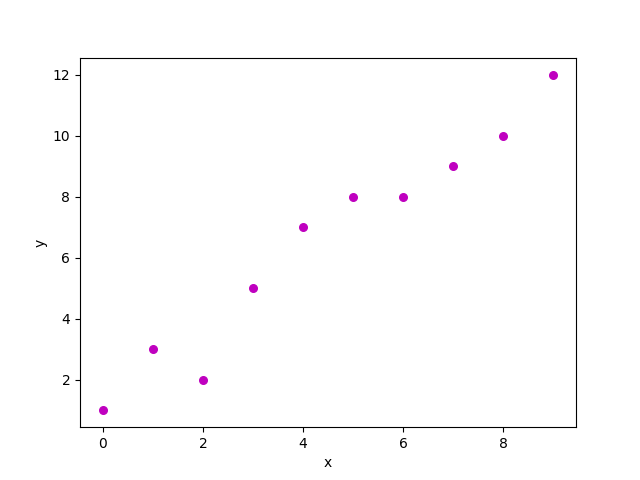
Being $\beta_0$ and $\beta_1$ the intercept and slope of a linear function, and $\epsilon$ an error term. Relationship between $x$ and $y$ can be expressed as follows:

$y_i = \beta_0 + \beta_1 x_i + \epsilon_i ~~~~~ \textrm{with}~i=1,2,3,...n$

That can also be expressed in matricial form.

$Y = \beta_0 + \beta_1 X + \epsilon = \beta [1|X] + \epsilon ~~~~~ \textrm{with}~\beta = \begin{bmatrix}\beta_0&\beta_1\end{bmatrix}$

Where $X$ and $Y$ are $n$ -element column vectors and $[1|X]$ is a column vector of ones padded to the left side of $X$

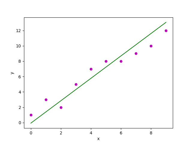
Given such representation, $\beta$ terms can be estimated by applying the following formula based on least-square optimization:

$\beta = (X^TX)^{-1}X^Ty$

From that, $\beta$ coefficients can be used to create a linear estimator and predict new instances of $x$ as shown in the following plot.

Problem¶

The following dataset includes data about the poverty rate (PovPct) and the birth rate for women between 15 and 17 years old (Brth15to17) for 50 states and the District of Columbia in United States.

You are asked to use least-square optimization to create a linear estimator able to predict the birth rate of a community based on the poverty rate associated to it.

In [9]:

import matplotlib.pyplot as plt
import urllib2,ssl

#Anulate https verification process
ssl._create_default_https_context = ssl._create_unverified_context

#load data from web source
data_link = urllib2.urlopen("https://onlinecourses.science.psu.edu/stat462/sites/onlinecourses.science.psu.edu.stat462/files/data/poverty/index.txt")
data = np.genfromtxt(data_link,delimiter='\t',skip_header=1)[:,1:3] #load only PovPct and Brth15to17 columns

plt.figure(figsize=(8,5))
plt.plot(data[:,0],data[:,1],'ro')
plt.xlabel("Poverty rate")
plt.ylabel("Birth rate (15-17 years)")
plt.grid(True)
plt.show()

<Figure size 800x500 with 1 Axes>

In [10]:

###########################
### HERE GOES YOUR CODE ###
# 1. Extract subsets from 'data' to create the vector 'X' and 'Y' corresponding to 'PovPct' and 'Brth15to17'.
# 2. Concatenate a column of ones to the left side of X
# 3. Use least square regression formula to estimate the two linear coefficients into a 2x1 array called 'beta'
# 4. Estimate predictions 'Y_pred' from X, using Y_pred = beta[0] + beta[1]X
# 5. Plot results using same instructions as above, just uncomment "plt.plot(data[:,0],Y_pred,'g-')" line below
###########################



plt.figure(figsize=(8,5))
plt.plot(data[:,0],data[:,1],'ro')
#plt.plot(data[:,0],Y_pred,'g-')
plt.xlabel("Poverty rate")
plt.ylabel("Birth rate (15-17 years)")
plt.grid(True)
plt.show()