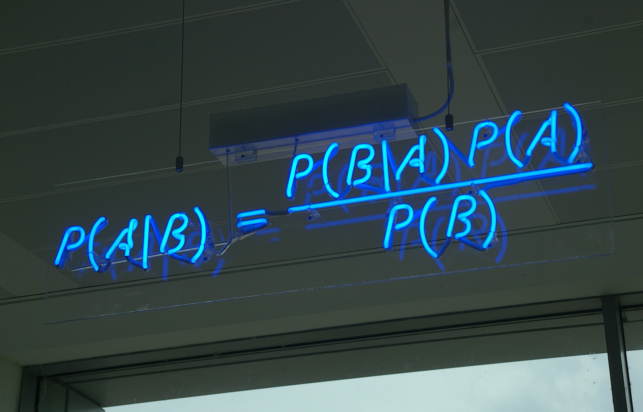
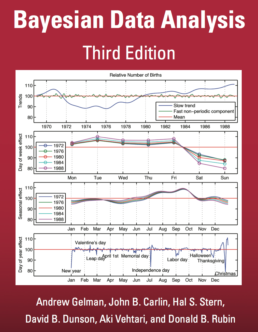
To build these slides:
%%bash
jupyter nbconvert \
    --to=slides \
    --reveal-prefix=https://cdnjs.cloudflare.com/ajax/libs/reveal.js/3.2.0/ \
    --output=dataphilly-jul2016 \
    ./DataPhilly\ July\ 2016\ Introduction\ to\ Probabilistic\ Programming.ipynb
[NbConvertApp] Converting notebook ./DataPhilly July 2016 Introduction to Probabilistic Programming.ipynb to slides
[NbConvertApp] Writing 561178 bytes to ./dataphilly-jul2016.slides.html
%matplotlib inline
from __future__ import division
from IPython.display import Image
from matplotlib import pyplot as plt
import numpy as np
import pandas as pd
import scipy as sp
import seaborn as sns
from theano import tensor as T
blue, green, red, purple, gold, teal = sns.color_palette()
plt.rc('figure', figsize=(8, 6))

LABELSIZE = 14
plt.rc('axes', labelsize=LABELSIZE)
plt.rc('legend', fontsize=LABELSIZE)
plt.rc('xtick', labelsize=LABELSIZE)
plt.rc('ytick', labelsize=LABELSIZE)
SEED = 2285280 # from random.org
Introduction to Probabilistic Programming
DataPhilly
July 13, 2016
@Austin Rochford (arochford@monetate.com)
Probabilistic Programming
- Programming with random variables
- User specifies a generative model for the observed data
- "Tell the story" of how the data were created
- The language runtime/software library automatically performs inference

What do we mean by inference?
- Maximum likelihood inference
- Maxumum a posteriori inference
- Full posterior inference

Disease Testing
A certain rare disease affects one in 10,000 people. A test for the disease gives the correct result 99.9% of the time.
What is the probability that a given test is positive?
import pymc3 as pm

with pm.Model() as pretest_disease_model:
    # This is our prior belief about whether or not the subject has the disease,
    # given its prevalence of the disease in the general population
    has_disease = pm.Bernoulli('has_disease', 1e-4)

    # This is the probability of a positive test given the presence or lack
    # of the disease
    p_positive = pm.Deterministic('p_positive',
                                  T.switch(T.eq(has_disease, 1),
                                           # If the subject has the disease,
                                           # this is the probability that the
                                           # test is positive
                                           0.999,
                                           # If the subject does not have the
                                           # disease, this is the probability
                                           # that the test is negative
                                           1 - 0.999))

    # This is the observed test result
    test_positive = pm.Bernoulli('test_positive', p_positive)
samples = 40000
with pretest_disease_model:
    step = pm.Metropolis()
    pretest_disease_trace = pm.sample(samples, step, random_seed=SEED)
[-----------------100%-----------------] 40000 of 40000 complete in 6.1 sec
pretest_disease_trace['test_positive']
array([0, 0, 0, ..., 0, 0, 0])
pretest_disease_trace['test_positive'].size
40000
The probability that a given test is positive is
pretest_disease_trace['test_positive'].mean()
0.001575
0.999 * 1e-4 + (1 - 0.999) * (1 - 1e-4)
0.0010998000000000008
If a subject tests positive, what is the probability they have the disease?
with pm.Model() as disease_model:
    # This is our prior belief about whether or not the subject has the disease,
    # given its prevalence of the disease in the general population
    has_disease = pm.Bernoulli('has_disease', 1e-4)

    # This is the probability of a positive test given the presence or lack
    # of the disease
    p_positive = pm.Deterministic('p_positive',
                                  T.switch(T.eq(has_disease, 1),
                                           # If the subject has the disease,
                                           # this is the probability that the
                                           # test is positive
                                           0.999,
                                           # If the subject does not have the
                                           # disease, this is the probability
                                           # that the test is negative
                                           1 - 0.999))

    # This is the observed positive test
    test_positive = pm.Bernoulli('test_positive', p_positive, observed=1)
with disease_model:
    step = pm.Metropolis()
    disease_trace = pm.sample(samples, step, random_seed=SEED)
[-----------------100%-----------------] 40000 of 40000 complete in 3.8 sec
The probability that someone who tests positive for the disease has it is
disease_trace['has_disease'].mean()
0.096775
0.999 * 1e-4 / (0.999 * 1e-4 + (1 - 0.999) * (1 - 1e-4))
0.09083469721767587
The Monty Hall Problem

If we select the first door and Monty opens the third to reveal a goat, should we change doors?
with pm.Model() as monty_model:
    # We have no idea where the prize is at the beginning
    prize = pm.DiscreteUniform('prize', 0, 2)

    # The probability that Monty opens each door
    p_open = pm.Deterministic('p_open',
                              T.switch(T.eq(prize, 0),
                                       # If the prize is behind the first door,
                                       # he chooses to open one of the others
                                       # at random
                                       np.array([0., 0.5, 0.5]),
                                       T.switch(T.eq(prize, 1),
                                                # If it is behind the second door,
                                                # he must open the third door
                                                np.array([0., 0., 1.]),
                                                # If it is behind the third door,
                                                # he must open the second door
                                                np.array([0., 1., 0.]))))

    # Monty opened the third door, revealing a goat
    opened = pm.Categorical('opened', p_open, observed=2)
samples = 10000
with monty_model:
    step = pm.Metropolis()
    monty_trace = pm.sample(samples, step, random_seed=SEED)

monty_trace_df = pm.trace_to_dataframe(monty_trace)
[-----------------100%-----------------] 10000 of 10000 complete in 1.4 sec
monty_trace_df.head()
| p_open__0 | p_open__1 | p_open__2 | prize | |
|---|---|---|---|---|
| 0 | 0.0 | 0.0 | 1.0 | 1 |
| 1 | 0.0 | 0.5 | 0.5 | 0 |
| 2 | 0.0 | 0.0 | 1.0 | 1 |
| 3 | 0.0 | 0.0 | 1.0 | 1 |
| 4 | 0.0 | 0.0 | 1.0 | 1 |
(monty_trace_df.groupby('prize')
               .size()
               .div(monty_trace_df.shape[0]))
prize
0    0.3196
1    0.6804
dtype: float64
Built on top of theano
- Dynamic generation of
Ccode for models - Automatic differentiation allows for gradient-based inference
- Implements advanced Markov chain Monte carlo algorithms, such at the No U-Turn Sampler
- Implements automatic differentiation variational inference
- Interoperable with both
pandasandpatsy - Provides clean support for multilevel models

A/B Testing

Suppose variant A sees 510 visitors and 40 purchases, but variant B sees 505 visitors and 50 conversions.
with pm.Model() as ab_model:
    # A priori, we have no idea what the purchase rate for variant A will be
    a_rate = pm.Uniform('a_rate')
    # We observed 40 purchases from 510 visitors who saw variant A
    a_purchases = pm.Binomial('a_purchases', 510, a_rate, observed=40)

    # A priori, we have no idea what the purchase rate for variant B will be
    b_rate = pm.Uniform('b_rate')
    # We observed 40 purchases from 510 visitors who saw variant A
    b_purchases = pm.Binomial('b_purchases', 505, b_rate, observed=45)
Applied interval-transform to a_rate and added transformed a_rate_interval to model.
Applied interval-transform to b_rate and added transformed b_rate_interval to model.
samples = 10000
with ab_model:
    step = pm.NUTS()
    ab_trace = pm.sample(samples, step, random_seed=SEED)
[-----------------100%-----------------] 10000 of 10000 complete in 3.2 sec
fig, ax = plt.subplots(figsize=(8, 6))

BINS = 30

ax.hist(np.clip(ab_trace['a_rate'], 0.03, 0.15),
        bins=BINS, normed=True, lw=0, alpha=0.75,
        label="Variant A");
ax.hist(np.clip(ab_trace['b_rate'], 0.03, 0.15),
        bins=BINS, normed=True, lw=0, alpha=0.75,
        label="Variant B");

ax.set_xlabel('Purchase rate');
ax.set_yticklabels([]);
ax.legend();
fig
The probability that variant B is better than variant A is
(ab_trace['a_rate'] < ab_trace['b_rate']).mean()
0.7218
Robust Regression
x = np.array([10, 8, 13, 9, 11, 14, 6, 4, 12, 7, 5])
y = np.array([7.46, 6.77, 12.74, 7.11, 7.81, 8.84, 6.08, 5.39, 8.15, 6.42, 5.73])
fig, ax = plt.subplots(figsize=(8, 6))

ax.scatter(x, y, c='k', s=50);
fig
X = np.empty((x.size, 2))
X[:, 0] = 1
X[:, 1] = x

coef, _, __, ___ = np.linalg.lstsq(X, y)
plot_X = np.ones((100, 2))

x_min, x_max = x.min() - 1, x.max() + 1
plot_X[:, 1] = np.linspace(x_min, x_max, 100)
fig, ax = plt.subplots(figsize=(8, 6))

ax.scatter(x, y, c='k', s=50);
ax.plot(plot_X[:, 1], plot_X.dot(coef),
        c='k', label='Least squares');

ax.set_xlim(x_min, x_max);
ax.legend(loc=2);
fig
with pm.Model() as ols_model:
    # alpha is the slope and beta is the intercept
    alpha = pm.Uniform('alpha', -100, 100)
    beta = pm.Uniform('beta', -100, 100)

    # Ordinary least squares assumes that the noise is normally distributed
    y_obs = pm.Normal('y_obs', alpha + beta * x, 1., observed=y)
Applied interval-transform to alpha and added transformed alpha_interval to model.
Applied interval-transform to beta and added transformed beta_interval to model.
samples = 10000
with ols_model:
    step = pm.Metropolis()
    ols_trace = pm.sample(samples, step, random_seed=SEED)
[-----------------100%-----------------] 10000 of 10000 complete in 2.2 sec
post_y = ols_trace['alpha'] + np.outer(plot_X[:, 1], ols_trace['beta'])
fig, ax = plt.subplots(figsize=(8, 6))

ax.fill_between(plot_X[:, 1],
                np.percentile(post_y, 2.5, axis=1),
                np.percentile(post_y, 97.5, axis=1),
                color='gray', alpha=0.5,
                label='95% CI');
ax.scatter(x, y, c='k', s=50);
ax.plot(plot_X[:, 1], plot_X.dot(coef),
        c='k', label='Least squares');
ax.plot(plot_X[:, 1], post_y.mean(axis=1),
        c='r', ls='--', label='PyMC3 least squares');

ax.set_xlim(x_min, x_max);
ax.legend(loc=2);
fig
fig, ax = plt.subplots(figsize=(8, 6))

z = np.linspace(-4, 4, 100)

ax.plot(z, sp.stats.norm.pdf(z),
        label='$N(0, 1)$');
ax.plot(z, sp.stats.t.pdf(z, 3),
        label=r'$t(\nu = 3)$');

ax.set_xlabel('Residual');
ax.set_yticklabels([]);
ax.set_ylabel('Probability density');
ax.legend();
fig
with pm.Model() as robust_model:
    # alpha is the slope and beta is the intercept
    alpha = pm.Uniform('alpha', -100, 100)
    beta = pm.Uniform('beta', -100, 100)

    # t-distributed residuals are less sensitive to outliers
    y_obs = pm.StudentT('y_obs', nu=3., mu=alpha + beta * x, observed=y)
Applied interval-transform to alpha and added transformed alpha_interval to model.
Applied interval-transform to beta and added transformed beta_interval to model.
with robust_model:
    step = pm.Metropolis()

    robust_trace = pm.sample(samples, step, random_seed=SEED)
[-----------------100%-----------------] 10000 of 10000 complete in 2.3 sec
post_y_robust = robust_trace['alpha'] + np.outer(plot_X[:, 1], robust_trace['beta'])
fig, (l_ax, r_ax) = plt.subplots(ncols=2, sharex=True, sharey=True, figsize=(16, 6))

l_ax.fill_between(plot_X[:, 1],
                  np.percentile(post_y, 2.5, axis=1),
                  np.percentile(post_y, 97.5, axis=1),
                  color='gray', alpha=0.5,
                  label='95% CI');
l_ax.scatter(x, y, c='k', s=50);
l_ax.plot(plot_X[:, 1], plot_X.dot(coef),
          c='k', label='Least squares');
l_ax.plot(plot_X[:, 1], post_y.mean(axis=1),
          c='r', ls='--', label='PyMC3 least squares');

l_ax.set_xlim(x_min, x_max);
l_ax.legend(loc=2);

r_ax.fill_between(plot_X[:, 1],
                  np.percentile(post_y_robust, 2.5, axis=1),
                  np.percentile(post_y_robust, 97.5, axis=1),
                  color='gray', alpha=0.5,
                  label='95% CI');
r_ax.scatter(x, y, c='k', s=50);
r_ax.plot(plot_X[:, 1], post_y_robust.mean(axis=1),
          c=blue, label='PyMC3 robust');

r_ax.set_xlim(x_min, x_max);
r_ax.legend(loc=2);
fig
Congressional Ideal Point Model
vote_data_uri = 'http://archive.ics.uci.edu/ml/machine-learning-databases/voting-records/house-votes-84.data'
N_BILLS = 16
BILLS = list(range(N_BILLS))

df = pd.read_csv(vote_data_uri, names=['party'] + BILLS)

df.index.name = 'rep'

df[df == 'n'] = 0
df[df == 'y'] = 1
df[df == '?'] = np.nan

df.party, parties = df.party.factorize()

N_REPS = df.shape[0]
df.head()
| party | 0 | 1 | 2 | 3 | 4 | 5 | 6 | 7 | 8 | 9 | 10 | 11 | 12 | 13 | 14 | 15 | |
|---|---|---|---|---|---|---|---|---|---|---|---|---|---|---|---|---|---|
| rep | |||||||||||||||||
| 0 | 0 | 0 | 1 | 0 | 1 | 1 | 1 | 0 | 0 | 0 | 1 | NaN | 1 | 1 | 1 | 0 | 1 |
| 1 | 0 | 0 | 1 | 0 | 1 | 1 | 1 | 0 | 0 | 0 | 0 | 0 | 1 | 1 | 1 | 0 | NaN |
| 2 | 1 | NaN | 1 | 1 | NaN | 1 | 1 | 0 | 0 | 0 | 0 | 1 | 0 | 1 | 1 | 0 | 0 |
| 3 | 1 | 0 | 1 | 1 | 0 | NaN | 1 | 0 | 0 | 0 | 0 | 1 | 0 | 1 | 0 | 0 | 1 |
| 4 | 1 | 1 | 1 | 1 | 0 | 1 | 1 | 0 | 0 | 0 | 0 | 1 | NaN | 1 | 1 | 1 | 1 |
parties
Index(['republican', 'democrat'], dtype='object')
vote_df = (pd.melt(df.reset_index(),
                   id_vars=['rep', 'party'], value_vars=BILLS,
                   var_name='bill', value_name='vote')
             .dropna()
             .astype(np.int64))
grid = sns.factorplot('bill', 'vote', 'party', vote_df,
                      kind='bar', ci=None, size=8, aspect=1.5);
grid.set_axis_labels('Bill', 'Percent voting for bill');
grid.fig
$p_{i, j}$ is the probability that representative $i$ votes for bill $j$.
$$ \begin{align*} \log \left(\frac{p_{i, j}}{1 - p_{i, j}}\right) & = \gamma_j \left(\alpha_i - \beta_j\right) \\ & = \textrm{ability of bill } j \textrm{ to discriminate} \times (\textrm{conservativity of represetative } i\ - \textrm{conservativity of bill } j) \end{align*} $$with pm.Model() as ideal_point_model:
# The conservativity of representative i
alpha = pm.Normal('alpha', 0, 1., shape=N_REPS)
# The conservativity of bill j
mu_beta = pm.Normal('mu_beta', 0, 1e-3)
sigma_beta = pm.Uniform('sigma_beta', 0, 1e2)
beta = pm.Normal('beta', mu_beta, sd=sigma_beta, shape=N_BILLS)
# The ability of bill j to discriminate
mu_gamma = pm.Normal('mu_gamma', 0, 1e-3)
sigma_gamma = pm.Uniform('sigma_gamma', 0, 1e2)
gamma = pm.Normal('gamma', mu_gamma, sd=sigma_gamma, shape=N_BILLS)
# The probability that representative i votes for bill j
p = pm.Deterministic('p', T.nnet.sigmoid(gamma[vote_df.bill] * (alpha[vote_df.rep] - beta[vote_df.bill])))
# The observed votes
vote = pm.Bernoulli('vote', p, observed=vote_df.vote)
Applied interval-transform to sigma_beta and added transformed sigma_beta_interval to model.
Applied interval-transform to sigma_gamma and added transformed sigma_gamma_interval to model.
samples = 20000
with ideal_point_model:
    step = pm.Metropolis()
    ideal_point_trace = pm.sample(samples, step, random_seed=SEED)
[-----------------100%-----------------] 20000 of 20000 complete in 107.5 sec
rep_alpha = ideal_point_trace['alpha'].mean(axis=0)
fig, ax = plt.subplots(figsize=(8, 6))

ax.hist(rep_alpha[(df.party == (parties == 'republican').argmax()).values],
        normed=True, bins=10, color=red, alpha=0.75, lw=0,
        label='Republicans');
ax.hist(rep_alpha[(df.party == (parties == 'democrat').argmax()).values],
        normed=True, bins=10, color=blue, alpha=0.75, lw=0,
        label='Democrats');

ax.set_xlabel(r'$\alpha$');
ax.set_yticklabels([]);
ax.set_ylabel('Probability density');
ax.legend(loc=1);
fig
pm.forestplot(ideal_point_trace, varnames=['gamma']);

Source: http://mqscores.berkeley.edu/
References
Probabilistic Programming and Bayesian Methods for Hackers (Open source, uses PyMC2, PyMC3 port in progress)
Think Bayes (Available freely online, calculations in Python)


