A Dockerfile that will produce a container with all the dependencies necessary to run this notebook is available here.
In [1]:
%matplotlib inline
In [2]:
import datetime
import logging
from warnings import filterwarnings
In [3]:
import arviz as az
from matplotlib import pyplot as plt
from matplotlib.ticker import StrMethodFormatter
import numpy as np
import pandas as pd
import pymc3 as pm
import scipy as sp
import seaborn as sns
from sklearn.preprocessing import LabelEncoder
from theano import pprint
WARNING (theano.configdefaults): install mkl with `conda install mkl-service`: No module named 'mkl'
In [4]:
sns.set(color_codes=True)
pct_formatter = StrMethodFormatter('{x:.1%}')
In [5]:
# configure pyplot for readability when rendered as a slideshow and projected
FIG_WIDTH, FIG_HEIGHT = 8, 6
plt.rc('figure', figsize=(FIG_WIDTH, FIG_HEIGHT))

LABELSIZE = 14
plt.rc('axes', labelsize=LABELSIZE)
plt.rc('axes', titlesize=LABELSIZE)
plt.rc('figure', titlesize=LABELSIZE)
plt.rc('legend', fontsize=LABELSIZE)
plt.rc('xtick', labelsize=LABELSIZE)
plt.rc('ytick', labelsize=LABELSIZE)
In [6]:
filterwarnings('ignore', 'findfont')
filterwarnings('ignore', "Conversion of the second argument of issubdtype")
filterwarnings('ignore', "Set changed size during iteration")

# keep theano from complaining about compile locks for small models
(logging.getLogger('theano.gof.compilelock')
        .setLevel(logging.CRITICAL))
In [7]:
SEED = 54902 # from random.org, for reproducibility

np.random.seed(SEED)

In [8]:
%%bash
DATA_URI=https://raw.githubusercontent.com/polygraph-cool/last-two-minute-report/32f1c43dfa06c2e7652cc51ea65758007f2a1a01/output/all_games.csv
DATA_DEST=/tmp/all_games.csv

if [[ ! -e $DATA_DEST ]];
then
    wget -q -O $DATA_DEST $DATA_URI
fi
In [9]:
USECOLS = [
    'period',
    'seconds_left',
    'call_type',
    'committing_player',
    'disadvantaged_player',
    'review_decision',
    'play_id',
    'away',
    'home',
    'date',
    'score_away',
    'score_home',
    'disadvantaged_team',
    'committing_team'
]
In [10]:
orig_df = pd.read_csv(
    '/tmp/all_games.csv',
    usecols=USECOLS,
    index_col='play_id',
    parse_dates=['date']
)
In [11]:
orig_df.head(n=2).T
Out[11]:
| play_id | 20150301CLEHOU-0 | 20150301CLEHOU-1 |
|---|---|---|
| period | Q4 | Q4 |
| seconds_left | 112 | 103 |
| call_type | Foul: Shooting | Foul: Shooting |
| committing_player | Josh Smith | J.R. Smith |
| disadvantaged_player | Kevin Love | James Harden |
| review_decision | CNC | CC |
| away | CLE | CLE |
| home | HOU | HOU |
| date | 2015-03-01 00:00:00 | 2015-03-01 00:00:00 |
| score_away | 103 | 103 |
| score_home | 105 | 105 |
| disadvantaged_team | CLE | HOU |
| committing_team | HOU | CLE |
In [12]:
foul_df = orig_df[
    orig_df.call_type
           .fillna("UNKNOWN")
           .str.startswith("Foul")
]
In [13]:
FOULS = [
    f"Foul: {foul_type}"
    for foul_type in [
        "Personal",
        "Shooting",
        "Offensive",
        "Loose Ball",
        "Away from Play"
    ]
]
In [14]:
TEAM_MAP = {
    "NKY": "NYK",
    "COS": "BOS",
    "SAT": "SAS",
    "CHi": "CHI",
    "LA)": "LAC",
    "AT)": "ATL",
    "ARL": "ATL"
}

def correct_team_name(col):
    def _correct_team_name(df):
        return df[col].apply(lambda team_name: TEAM_MAP.get(team_name, team_name))

    return _correct_team_name
In [15]:
def date_to_season(date):
    if date >= datetime.datetime(2017, 10, 17):
        return '2017-2018'
    elif date >= datetime.datetime(2016, 10, 25):
        return '2016-2017'
    elif date >= datetime.datetime(2015, 10, 27):
        return '2015-2016'
    else:
        return '2014-2015'
In [16]:
clean_df = (foul_df.where(lambda df: df.period == "Q4")
                   .where(lambda df: (df.date.between(datetime.datetime(2016, 10, 25),
                                                      datetime.datetime(2017, 4, 12))
                                      | df.date.between(datetime.datetime(2015, 10, 27),
                                                       datetime.datetime(2016, 5, 30)))
                         )
                   .assign(
                       review_decision=lambda df: df.review_decision.fillna("INC"),
                       committing_team=correct_team_name('committing_team'),
                       disadvantged_team=correct_team_name('disadvantaged_team'),
                       away=correct_team_name('away'),
                       home=correct_team_name('home'),
                       season=lambda df: df.date.apply(date_to_season)
                    )
                   .where(lambda df: df.call_type.isin(FOULS))
                   .dropna()
                   .drop('period', axis=1)
                   .assign(call_type=lambda df: (df.call_type
                                                   .str.split(': ', expand=True)
                                                   .iloc[:, 1])))
In [17]:
player_enc = LabelEncoder().fit(
    np.concatenate((
        clean_df.committing_player,
        clean_df.disadvantaged_player
    ))
)
n_player = player_enc.classes_.size

season_enc = LabelEncoder().fit(
    clean_df.season
)
n_season = season_enc.classes_.size
In [18]:
df = (clean_df[['seconds_left']]
              .round(0)
              .assign(
                foul_called=1. * clean_df.review_decision.isin(['CC', 'INC']),
                player_committing=player_enc.transform(clean_df.committing_player),
                player_disadvantaged=player_enc.transform(clean_df.disadvantaged_player),
                score_committing=clean_df.score_home.where(
                    clean_df.committing_team == clean_df.home,
                    clean_df.score_away
                ),
                score_disadvantaged=clean_df.score_home.where(
                    clean_df.disadvantaged_team == clean_df.home,
                    clean_df.score_away
                ),
                season=season_enc.transform(clean_df.season)
              ))
In [19]:
df.head()
Out[19]:
| seconds_left | foul_called | player_committing | player_disadvantaged | score_committing | score_disadvantaged | season | |
|---|---|---|---|---|---|---|---|
| play_id | |||||||
| 20151028INDTOR-1 | 89.0 | 1.0 | 162 | 98 | 99.0 | 106.0 | 0 |
| 20151028INDTOR-2 | 73.0 | 0.0 | 36 | 358 | 106.0 | 99.0 | 0 |
| 20151028INDTOR-3 | 38.0 | 1.0 | 229 | 222 | 99.0 | 106.0 | 0 |
| 20151028INDTOR-4 | 30.0 | 0.0 | 229 | 98 | 99.0 | 106.0 | 0 |
| 20151028INDTOR-6 | 24.0 | 0.0 | 229 | 100 | 99.0 | 106.0 | 0 |
In [20]:
player_committing = df.player_committing.values
player_disadvantaged = df.player_disadvantaged.values

season = df.season.values
In [21]:
def hierarchical_normal(name, shape):
    Δ = pm.Normal(f'Δ_{name}', 0., 1., shape=shape)
    σ = pm.HalfNormal(f'σ_{name}', 5.)

    return pm.Deterministic(name, Δ * σ)
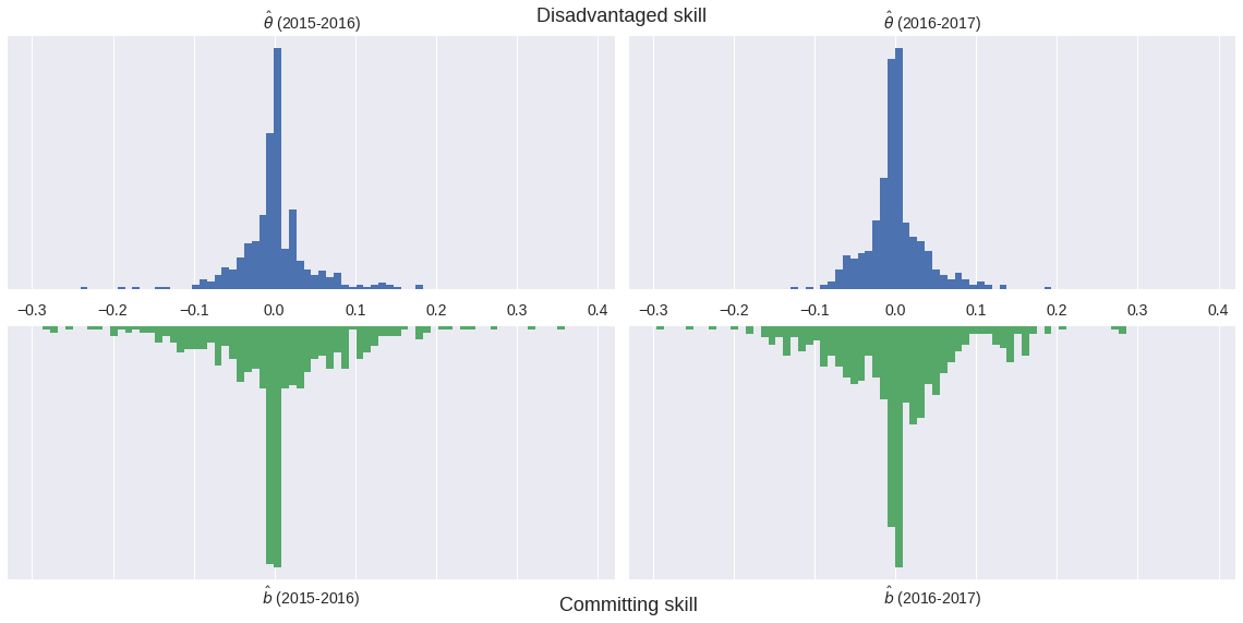
Model outline
$$ \operatorname{log-odds}(\textrm{Foul}) \ \sim \textrm{Season factor} + \left(\textrm{Disadvantaged skill} - \textrm{Committing skill}\right) $$In [22]:
with pm.Model() as irt_model:
β_season = pm.Normal('β_season', 0., 2.5, shape=n_season)
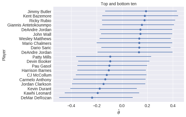
θ = hierarchical_normal('θ', n_player) # disadvantaged skill
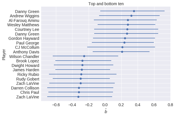
b = hierarchical_normal('b', n_player) # committing skill
p = pm.math.sigmoid(
β_season[season] + θ[player_disadvantaged] - b[player_committing]
)
obs = pm.Bernoulli(
'obs', p,
observed=df['foul_called'].values
)
In [23]:
CHAINS = 3

SAMPLE_KWARGS = {
    'chains': CHAINS,
    'cores': CHAINS,
    'random_seed': list(SEED + np.arange(CHAINS))
}
In [24]:
with irt_model:
    trace = pm.sample(500, **SAMPLE_KWARGS)
Auto-assigning NUTS sampler...
Initializing NUTS using jitter+adapt_diag...
Multiprocess sampling (3 chains in 3 jobs)
NUTS: [σ_b, Δ_b, σ_θ, Δ_θ, β_season]
Sampling 3 chains: 100%|██████████| 3000/3000 [02:07<00:00, 23.58draws/s]
In [25]:
az.plot_energy(trace);

In [26]:
az.rhat(trace).max()
Out[26]:
<xarray.Dataset>
Dimensions:   ()
Data variables:
    β_season  float64 1.0
    Δ_θ       float64 1.01
    Δ_b       float64 1.0
    σ_θ       float64 1.01
    θ         float64 1.01
    σ_b       float64 1.0
    b         float64 1.0
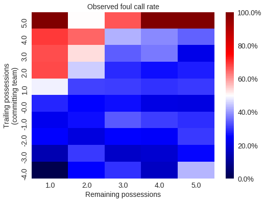
Basketball strategy leads to more complexity

In [27]:
df['trailing_committing'] = (df.score_committing
                               .lt(df.score_disadvantaged)
                               .mul(1.)
                               .astype(np.int64))
In [28]:
def make_foul_rate_yaxis(ax, label="Observed foul call rate"):
    ax.yaxis.set_major_formatter(pct_formatter)
    ax.set_ylabel(label)

    return ax
In [29]:
def make_time_axes(ax,
                   xlabel="Seconds remaining in game",
                   ylabel="Observed foul call rate"):
    ax.invert_xaxis()
    ax.set_xlabel(xlabel)

    return make_foul_rate_yaxis(ax, label=ylabel)
In [30]:
fig = make_time_axes(
    df.pivot_table('foul_called', 'seconds_left', 'trailing_committing')
      .rolling(20).mean()
      .rename(columns={0: "No", 1: "Yes"})
      .rename_axis("Committing team is trailing", axis=1)
      .plot()
).figure

In [31]:
fig
Out[31]:
The shot clock

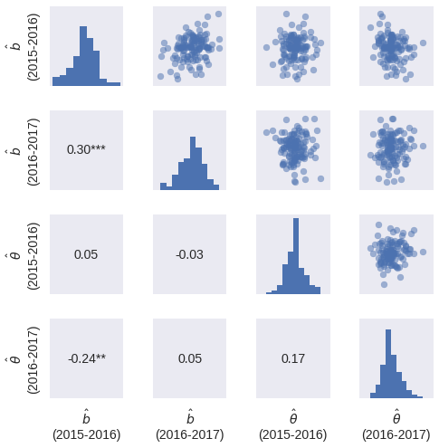
Are we measuring a skill?
|
|
Future Work
- Advanced baseball stats
- Hockey
- Faceoff skills
- Fighting ability

In [33]:
%%bash
jupyter nbconvert \
    --to=slides \
    --reveal-prefix=https://cdnjs.cloudflare.com/ajax/libs/reveal.js/3.2.0/ \
    --output=pp-sports-analytics-part-2 \
    ./basketball-irt.ipynb
[NbConvertApp] Converting notebook ./basketball-irt.ipynb to slides
[NbConvertApp] Writing 323016 bytes to ./pp-sports-analytics-part-2.slides.html
In [ ]: