Deep Learning in Action
Current state of AI
In the early days of artificial intelligence, the field rapidly tackled and solved problems that are intellectually difficult for human beings but relatively straightforward for computers - problems that can be described by a list of formal, mathematical rules. The true challenge to artificial intelligence proved to be solving the tasks that are easy for people to perform but hard for people to describe formally—problems that we solve intuitively, that feel automatic, like recognizing spoken words or faces in images.
Goodfellow et al. 2016, Deep Learning
Easy for us. Difficult for computers
- object recognition
- speech recognition
- speech generation
- labeling images
Representations matter
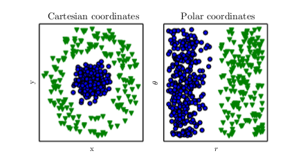
Just feed the network the right features?
- What are the correct pixel values for a "bike" feature?
- race bike, mountain bike, e-bike?
- pixels in the shadow may be much darker
- what if bike is mostly obscured by rider standing in front?
Let the network pick the features
... a layer at a time
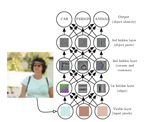
Deep Learning, 2 ways to think about it
- hierarchical feature extraction (start simple, end complex)
- function composition (see http://colah.github.io/posts/2015-09-NN-Types-FP/)
A Short History of (Deep) Learning
The first wave: cybernetics (1940s - 1960s)
- neuroscientific motivation
- linear models
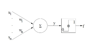
McCulloch-Pitts Neuron (MCP, 1943, a.k.a. Logic Circuit)
- binary output (0 or 1)
- neurons may have inhibiting (negative) and excitatory (positive) inputs
- each neuron has a threshold that has to be surpassed by the sum of activations for the neuron to get active (output 1)
- if just one input is inhibitory, the neuron will not activate

Perceptron (Rosenblatt, 1958): Great expectations
- compute linear combination of inputs
- return +1 if result is positive, -1 if result is negative
Minsky & Papert (1969), "Perceptrons": the great disappointment
- Perceptrons can only solve linearly separable problems
- Big loss of interest in neural networks
The second wave: Connectionism (1980s, mid-1990s)
- distributed representations
- backpropagation gets popular
The magic ingredient: backpropagation
Several "origins" in different fields, see e.g.
Henry J. Kelley (1960). Gradient theory of optimal flight paths. Ars Journal, 30(10), 947-954.
Arthur E. Bryson (1961, April). A gradient method for optimizing multi-stage allocation processes. In Proceedings of the Harvard Univ. Symposium on digital computers and their applications.
Paul Werbos (1974). Beyond regression: New tools for prediction and analysis in the behavioral sciences. PhD thesis, Harvard University.
Rumelhart, David E.; Hinton, Geoffrey E.; Williams, Ronald J. (8 October 1986). "Learning representations by back-propagating errors". Nature. 323 (6088): 533–536.
Backprop: How could the magic fail?
- Only applicable in case of supervised learning
- Doesn't scale well to multiple layers (as they thought at the time)
- Can converge to poor local minima (as they thought at the time)
The third wave: Deep Learning
- everything starts with: Hinton, G. E., Osindero, S., & Teh, Y. W. (2006). A fast learning algorithm for deep belief nets. Neural computation, 18(7), 1527-1554.
- deep neural networks can be trained efficiently, if the weights are initialized intelligently
- return of backpropagation
The architectures en vogue now (CNN, RNN, LSTM...) have mostly been around since the 1980s/1990s.
So why the hype success now?
Big data
It is true
that some skill is required to get good performance from a deep learning algorithm. Fortunately, the amount of skill required reduces as the amount of training data increases. The learning algorithms reaching human performance on complex tasks today are nearly identical to the learning algorithms that struggled to solve toy problems in the 1980s [...].
Goodfellow et al. 2016, Deep Learning
Dataset size - rule of thumb
As of 2016, a rough rule of thumb
is that a supervised deep learning algorithm will generally achieve acceptable performance with around 5,000 labeled examples per category, and will match or exceed human performance when trained with a dataset containing at least 10 million labeled examples.
Goodfellow et al. 2016, Deep Learning
Big models
thanks to faster/better
- hardware (CPUs, GPUs)
- network infrastructure
- software implementations
Since the introduction of hidden units, artificial neural networks have doubled in size roughly every 2.4 years.
Goodfellow et al. 2016, Deep Learning
Big impact
- deep networks consistently win prestigious competitions (e.g., ImageNet)
- deep learning solves increasingly complex problems (e.g., sequence-to-sequence learning)
- deep learning has started to fuel other research areas
and most importantly: Deep learning is highly profitable
Deep learning is now used by many top technology companies including Google, Microsoft, Facebook, IBM, Baidu, Apple, Adobe, Netflix, NVIDIA and NEC.
Goodfellow et al. 2016, Deep Learning
Deep Learning Architectures
Feedforward Deep Neural Network

Multi-layer Perceptron (MLP)
Caveat (terminology-related)
So “multi-layer” neural networks do not use the perceptron learning
procedure.
They should never have been called multi-layer perceptrons.
Geoffrey Hinton, Neural Networks for Machine Learning Lec. 3
What people mean by MLP is just a deep feedforward neural network.
Why hidden layers?
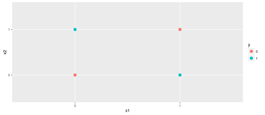
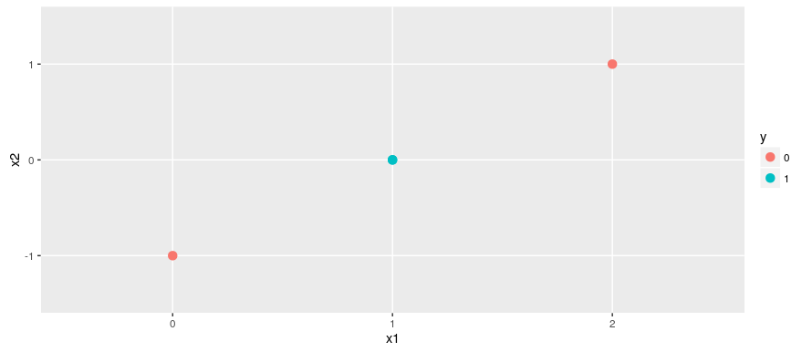
Learning XOR
We want to predict
- 0 from [0,0]
- 0 from [1,1]
- 1 from [0,1]
- 1 from [1,0]
Trying a linear model
$f(\mathbf{x}; \mathbf{w}, b) = \mathbf{x}^T\mathbf{w} + b$
- with Mean Squared Error cost (MSE), this leads to: $\mathbf{w}=0, b=0.5$
- mapping every point to 0.5!
Introduce hidden layer
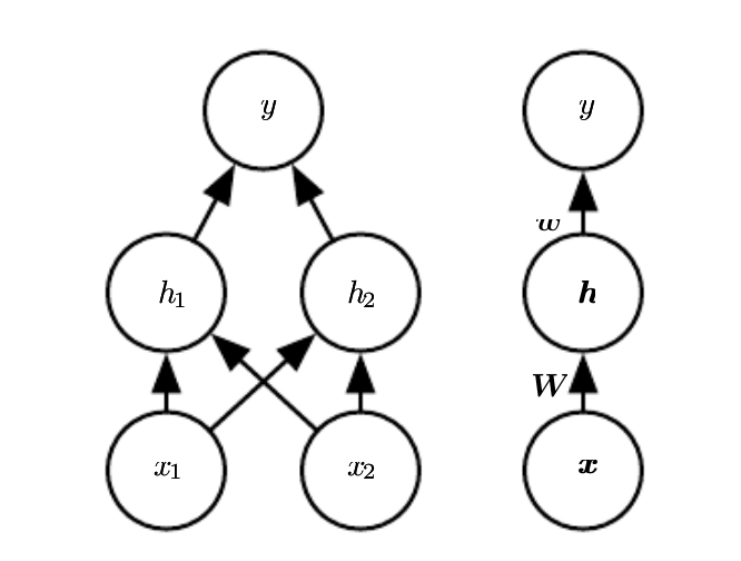
Calculation with hidden layer
$f(\mathbf{x}; \mathbf{W}, \mathbf{c}, \mathbf{w}, b) = \mathbf{w}^T (\mathbf{W}^T\mathbf{x} + \mathbf{c}) + b$
Design matrix: $\mathbf{X} = \begin{bmatrix}0 & 0 \\0 & 1\\1 & 0 \\1 & 1\end{bmatrix}$
Parameters: $\mathbf{W} = \begin{bmatrix}1 & 1 \\1 & 1\end{bmatrix}$, $\mathbf{c} = \begin{bmatrix}0 \\ -1 \end{bmatrix}$, $\mathbf{w} = \begin{bmatrix}1 \\ -2 \end{bmatrix}$
Input to hidden layer: $\mathbf{X}\mathbf{W} = \begin{bmatrix}0 & 0 \\1 & 1\\1 & 1 \\2 & 2\end{bmatrix}$, add $\mathbf{c}$ to every row ==> $\begin{bmatrix}0 & -1 \\1 & 0\\1 & 0 \\2 & 1\end{bmatrix}$
Which gives us...
Introducing nonlinearity
$f(\mathbf{x}; \mathbf{W}, \mathbf{c}, \mathbf{w}, b) = \mathbf{w}^T max(0, \mathbf{W}^T\mathbf{x} + \mathbf{c}) + b$
Output of rectified linear transformation: $\begin{bmatrix}0 & 0 \\1 & 0\\1 & 0 \\2 & 1\end{bmatrix}$

The remaining hidden-to-output transformation is linear, but the classes are already linearly separable.
How to train a deep network (1): Gradient Descent
Optimization
- Like other machine learning algorithms, neural networks learn by minimizing a cost function.
- Cost functions in neural networks normally are not convex and so, cannot be optimized in closed form.
- The solution is to do gradient descent.

Local minima

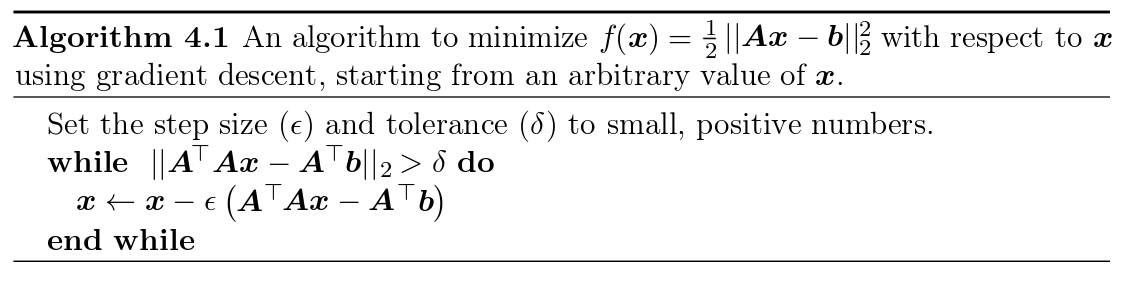
Closed-form vs. gradient descent optimization by example: Least Squares
Minimize squared error $f(\mathbf{x}) = ||\mathbf{X\hat{\beta} - y}||^2_2$
Closed form: solve normal equations $\mathbf{\hat{\beta}} = (\mathbf{X}^T\mathbf{{X}})^{-1} \mathbf{X}^T \mathbf{y}$
Alternatively, follow the gradient: $\nabla_x f(\mathbf{x})= \mathbf{X}^T\mathbf{X}\mathbf{\hat{\beta}} - \mathbf{X^Ty}$
This gives us a way to train one weight matrix.
How about a net with several layers?
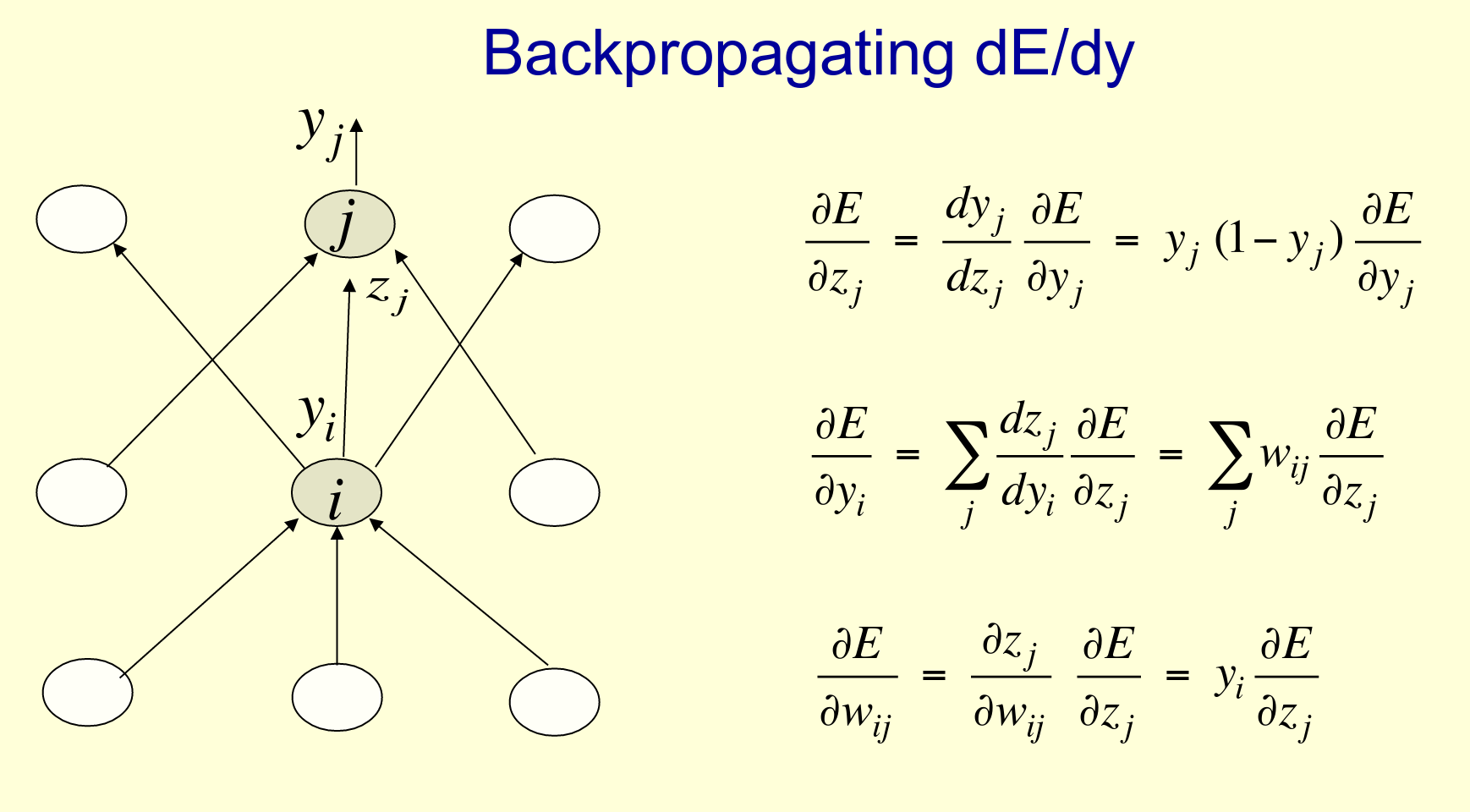
How to train a deep network (2): Backpropagation
Who else to ask but Geoff Hinton...
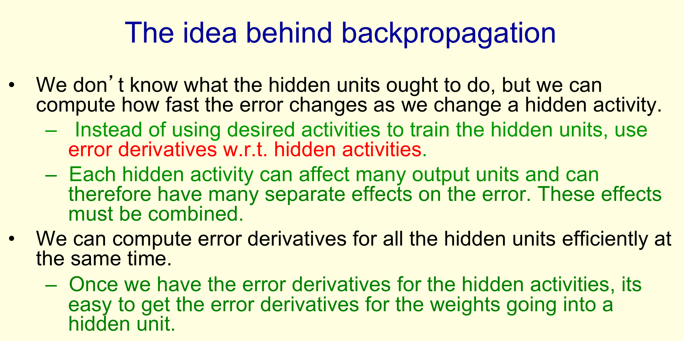
The mechanics of backprop
- basically, just the chain rule: $\frac{dz}{dx} = \frac{dz}{dy} \frac{dy}{dx}$
- chained over several layers:

Backprop example: logistic neuron
Decisions (1): Which loss function should I choose?
the loss (or cost) function indicates the cost incurred from false prediction / misclassification
probably the best-known loss function in machine learning is mean squared error:
$\frac{1}{n} \sum_n{(\hat{y} - y)^2}$
most of the time, in deep learning we use cross entropy:
$- \sum_j{t_j log(y_j)}$
This is the negative log probability of the right answer.
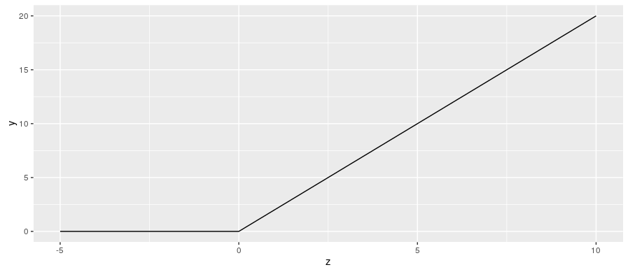
Decisions (2): Which activation function to choose?
purpose of activation function: introduce nonlinearity (see above)
for a long time, the sigmoid (logistic) activation function was used a lot:
$y = \frac{1}{1 + e^{-z}}$

now rectified linear units (ReLUs) are preferred:
$y = max(0, z)$
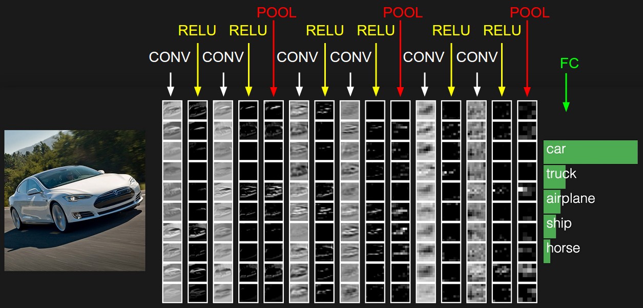
Convolutional Neural Networks
Why Conv Nets?
- conventional feedforward networks need equally sized input (images for example normally aren't!)
- convolution operation extracts image features
The Convolution Operation

Convolution and cross-correlation
- Strictly, the operation shown above (and implemented in most DL libraries) is not convolution, but cross-correlation
- 1-dimensional discrete convolution: $s(t) = (x * w)(t) = \sum_a{x(a) w(t-a)}$
- 2-dimensional convolution: $S(i,j) = I * K (i,j) = \sum_m \sum_n{I(m,n)K(i-m,j-n)}$
- 2-dimensional cross-correlation: $S(i,j) = I * K (i,j) = \sum_m \sum_n{I(i+m,j+n)K(m,n)}$
Octave demo
A = [1,2,3;4,5,6;7,8,9] # input "image"
# padded input matrix, for easier visualization
A_padded = [zeros(1,size(A,2)+2); [zeros(size(A,1),1), A, zeros(size(A,1),1)]; zeros(1,size(A,2)+2)]
B = [1,0;0,0] # kernel

# real convolution
C_full = conv2(A,B,'full') # default
C_same = conv2(A,B,'same')
C_valid = conv2(A,B,'valid')

# cross-correlation
XC = xcorr2(A,B)
Gimp demo
- Edge enhance: $\begin{bmatrix}0 & 0 & 0\\-1 & 1 & 0\\0 & 0 & 0\end{bmatrix}$, edge detect: $\begin{bmatrix}0 & 1 & 0\\1 & -4 & 1\\0 & 1 & 0\end{bmatrix}$
- Blur: $\begin{bmatrix}1 & 1 & 1\\1 & 1 & 1\\1 & 1 & 1\end{bmatrix}$, sharpen: $\begin{bmatrix}0 & -1 & 0\\-1 & 5 & -1\\0 & -1 & 0\end{bmatrix}$
Language modeling and word vectors
Language modeling
- predict next word given preceding ones
- based on statistical properties of the distribution of sequences of words
Distributional hypothesis: linguistic items with similar distributions have similar meanings
- n-gram/count-based (e.g., Latent Semantic Analysis)
- predictive (neural network language models, e.g., word2vec)
ngram-based
- choose ngram-size n
- estimate the probability $P(w_{t+1}|w_1,...,w_{t−2},w_{t−1},w_t)$ by ignoring context beyond n−1 words and dividing by the count of all given words up till $w_t$
- e.g., with bigrams: $P(w_{t+1}|w_t = \frac{count(w_{t+1},w_t)}{count(w_t)})$
neural network example (Bengio et al 2001, Bengio et al 2003)
- choose a context size n, as in ngrams
- map each word $w_{t−i}$ in the $n-1$ - word context to an associated d-dimensional feature vector $C_{w_{t-i}}$
- predict next word using standard NN architecture with tanh (hidden layer) resp. softmax (output layer) activation functions
- train network to maximize log likelihood $L(θ)=\sum_t{log P(w_t|w_{t−n+1}, ..., w_{t−1}})$ using stochastic gradient descent
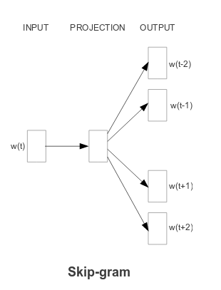
Word embeddings: word2vec
Mikolov et al (2013a). Efficient estimation of word representations in vector space. arXiv:1301.3781.
- Continuous Bag of Words (CBOW)
- Skip-Gram
Continuous Bag of Words

Skip-gram
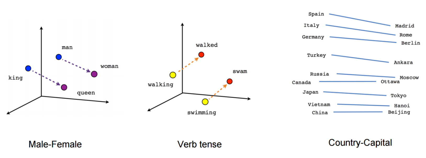
Semantic & syntactic relationships

word2vec visualizations
Recurrent neural networks (RNNs)
Why have recursion ?
- cannot process sequential data with "normal" feedforward networks
- in NLP, the n-gram approach cannot handle long-term relationships
Jane walked into the room. John walked in too. It was late in the
day, and everyone was walking home after a long day at work. Jane said hi to ___
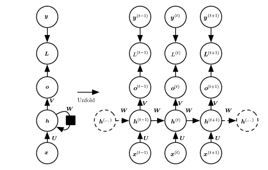
Two representations of RNNs
The recursion: example code
def rnn_cell(rnn_input, state):
    with tf.variable_scope('rnn_cell', reuse=True):
        W = tf.get_variable('W', [num_classes + state_size, state_size])
        b = tf.get_variable('b', [state_size], initializer=tf.constant_initializer(0.0))
    return tf.tanh(tf.matmul(tf.concat(1, [rnn_input, state]), W) + b)

state = init_state
rnn_outputs = []
for rnn_input in rnn_inputs:
    state = rnn_cell(rnn_input, state)
    rnn_outputs.append(state)
final_state = rnn_outputs[-1]
from: http://r2rt.com/recurrent-neural-networks-in-tensorflow-i.html
RNNs in practice: The need to forget
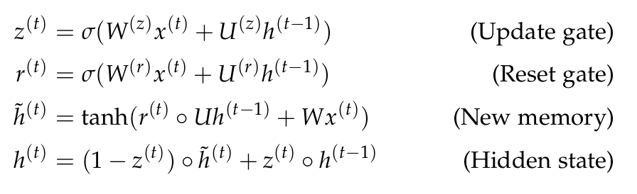
Gated Recurrent Units (GRUs)

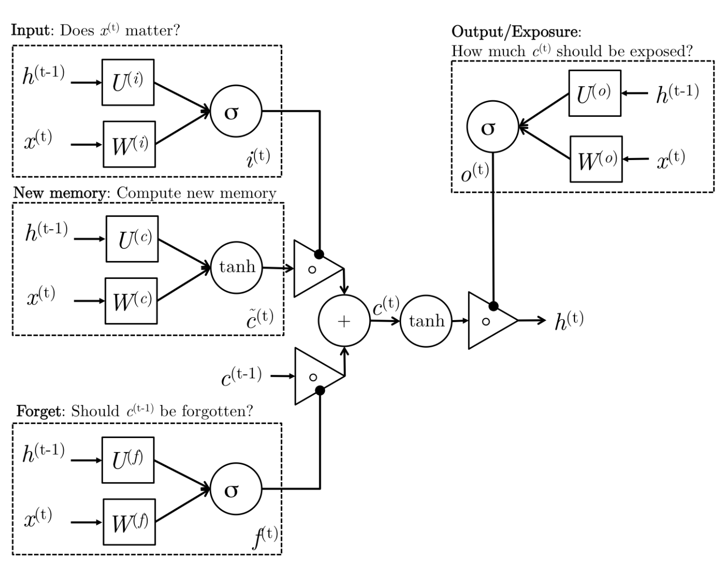
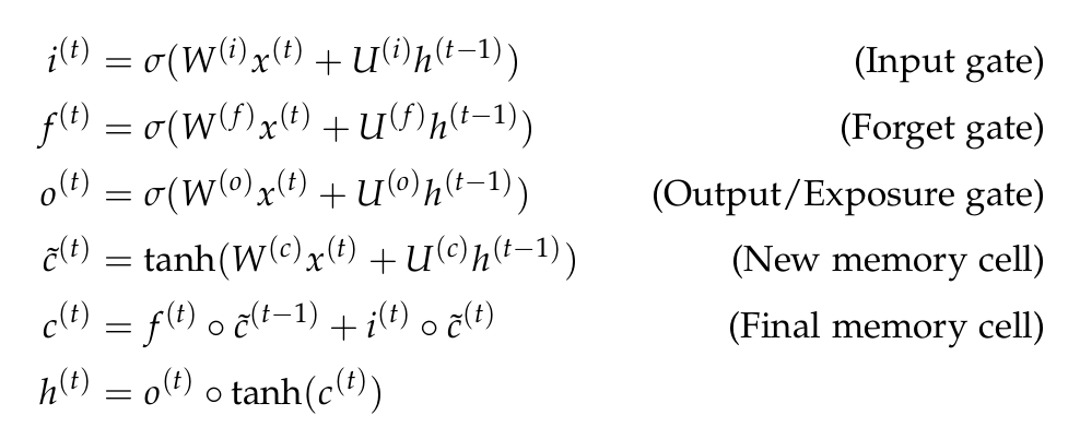
Long Short Term Memory (LSTM)
class BasicRNNCell(RNNCell):
  """The most basic RNN cell."""

  def __init__(self, num_units, input_size=None, activation=tanh):
    self._num_units = num_units
    self._activation = activation

  @property
  def state_size(self):
    return self._num_units

  def __call__(self, inputs, state, scope=None):
    """Most basic RNN: output = new_state = act(W * input + U * state + B)."""
    with vs.variable_scope(scope or "basic_rnn_cell"):
      output = self._activation(
          _linear([inputs, state], self._num_units, True, scope=scope))
return output, output
class GRUCell(RNNCell):
  """Gated Recurrent Unit cell (cf. http://arxiv.org/abs/1406.1078)."""

  def __call__(self, inputs, state, scope=None):
    """Gated recurrent unit (GRU) with nunits cells."""
    with vs.variable_scope(scope or "gru_cell"):
      with vs.variable_scope("gates"):  # Reset gate and update gate.
        # We start with bias of 1.0 to not reset and not update.
        r, u = array_ops.split(value=_linear([inputs, state],
                                             2 * self._num_units,
                                             True,
                                             1.0,
                                             scope=scope),
                               num_or_size_splits=2,
                               axis=1)
        r, u = sigmoid(r), sigmoid(u)

      with vs.variable_scope("candidate"):
        c = self._activation(_linear([inputs, r * state],
                                     self._num_units,
                                     True, scope=scope))

      new_h = u * state + (1 - u) * c

return new_h, new_h
class BasicLSTMCell(RNNCell):

  def __call__(self, inputs, state, scope=None):
    with vs.variable_scope(scope or "basic_lstm_cell"):

      c, h = array_ops.split(1, 2, state)
      concat = _linear([inputs, h], 4 * self._num_units, True, scope=scope)

      # i = input_gate, j = new_input, f = forget_gate, o = output_gate
      i, j, f, o = array_ops.split(1, 4, concat)

      new_c = (c * sigmoid(f + self._forget_bias) + sigmoid(i) * self._activation(j))
      new_h = self._activation(new_c) * sigmoid(o)

      new_state = array_ops.concat_v2([new_c, new_h], 1)
      return new_h, new_state
Mapping sequences to sequences: seq2seq
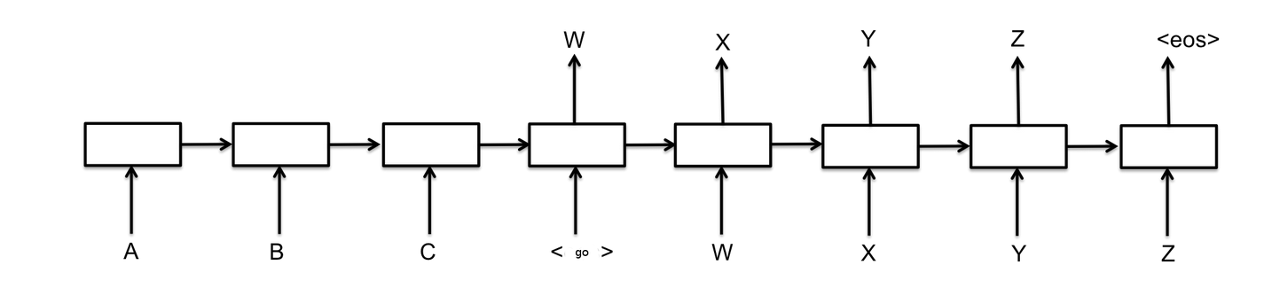
- first RNN encodes the input, second decodes the output
- applications: e.g., machine translation - though basically, all sequence-to-sequence translation!
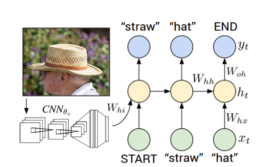
Combining modes/models example: Images and Descriptions
- Andrej Karpathy, Li Fei-Fei: Deep Visual-Semantic Alignments for Generating Image Descriptions
- combining CNNs, bidirectional RNNs, and multimodal embeddings
- Demo
Tensorflow Demo: Generating text
What is TensorFlow?
"If you can express your computation as a data flow graph, you can use TensorFlow."
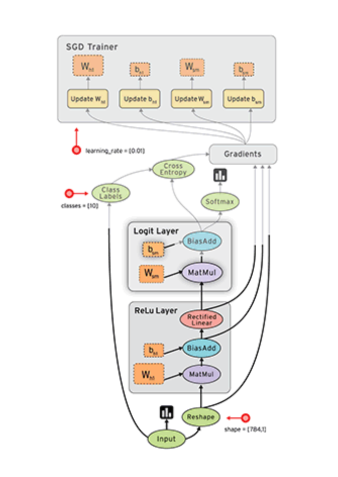
- represent computations as graphs
- nodes are operations
- edges are Tensors (multidimensional matrices) input to/output from operations
- to make anything happen, execute the graph in a Session
- a Session places and runs a graph on a Device (GPU, CPU)
Let's generate some text!
char-rnn demo
(based on https://github.com/sherjilozair/char-rnn-tensorflow)