This notebook contains course material from CBE20255 by Jeffrey Kantor (jeff at nd.edu); the content is available on Github. The text is released under the CC-BY-NC-ND-4.0 license, and code is released under the MIT license.
General Mass Balance on a Single Tank
Summary
This Jupyter notebook demonstrates the application of a mass balance to a simple water tank. This example is adapted with permission from learnCheme.com, a project at the University of Colorado funded by the National Science Foundation and the Shell Corporation.
Problem Statement
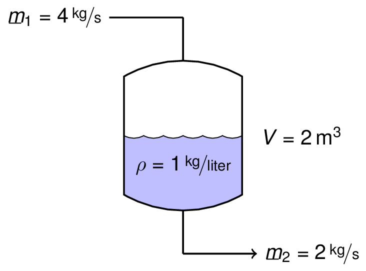
Draw a Diagram
Mass Balance
Using our general principles for a mass balance
$\frac{d(\rho V)}{dt} = \dot{m}_1 - \dot{m}_2$
which can be simplified to
$\frac{dV}{dt} = \frac{1}{\rho}\left(\dot{m}_1 - \dot{m}_2\right)$
where the initial value is $V(0) = 1\,\mbox{m}^3$. This is a differential equation.
Numerical Solution using odeint
import numpy as np
import matplotlib.pyplot as plt
%matplotlib inline

from scipy.integrate import odeint
# Flowrates in kg/sec
m1 = 4.0
m2 = 2.0

# Density in kg/m**3
rho = 1000.0

# Function to compute accumulation rate
def dV(V,t): return (m1 - m2)/rho;
Next we import odeint from the scipy.integrate package, set up a grid of times at which we wish to find solution values, then call odeint to compute values for the solution starting with an initial condition of 1.0.
t = np.linspace(0,1000)
V = odeint(dV,1.0,t)
We finish by plotting the results of the integration and comparing to the capacity of the tank.
plt.plot(t,V,'b',t,2*np.ones(len(t)),'r')
plt.xlabel('Time [sec]')
plt.ylabel('Volume [m**3]')
plt.legend(['Water Volume','Tank Capacity'],loc='upper left');

This same approach can be used solve systems of differential equations. For an light-hearted (but very useful) example, check out this solution for the Zombie Apocalypse.
Solving for the Time Required to Fill the Tank
Now that we know how to solve the differential equation, next we create a function to compute the air volume of the tank at any given time.
Vtank = 2.0
Vinitial = 1.0

def Vwater(t):
    return odeint(dV,Vinitial,[0,t])[-1][0]

def Vair(t):
    return Vtank - Vwater(t)

print("Air volume in the tank at t = 100 is {:4.2f} m**3.".format(Vair(100)))
Air volume in the tank at t = 100 is 0.80 m**3.
The next step is find the time at which Vair(t) returns a value of 0. This is root finding which the function brentq will do for us.
from scipy.optimize import brentq

t_full = brentq(Vair,0,1000)

print("The tank will be full at t = {:6.2f} seconds.".format(t_full))
The tank will be full at t = 500.00 seconds.
Exercise
Suppose the tank was being used to protect against surges in water flow, and the inlet flowrate was a function of time where
$\dot{m}_1 = 4 e^{-t/500}$
- Will the tank overflow?
- Assuming it doesn't overflow, how long would it take for the tank to return to its initial condition of being half full? To empty completely?
- What will be the peak volume of water in the tank, and when will that occur?