![]()
[T6] Advanced methods for neural end-to-end speech processing - unification, integration, and implementation -
Part4 : Building End-to-End TTS System
Speaker: Tomoki Hayashi
Department of informatics, Nagoya University
Human Dataware Lab. Co., Ltd.
Google colaboratory
- Online Jupyter notebook environment
- Can run python codes
- Can also run linux command with ! mark
- Can use a signal GPU (K80)
- What you need to use
- Internet connection
- Google account
- Chrome browser (recommended)

# example of the commands
print("hello, world.")
!echo "hello, world"
TOC
- Installation
- Introduction of ESPnet TTS
- Demonstration of the ESPnet TTS recipe
- Demonstration of the use of TTS pretrained models
- Demonstration of the use of ASR pretrained models
- Conclusion
0. Installation
It takes around 3 minutes. Please keep waiting for a while.
# OS setup
!cat /etc/os-release
!apt-get install -qq bc tree sox

# espnet setup
!pip install chainer==6.0.0
!git clone --depth 5 https://github.com/espnet/espnet -b v.0.9.7
!cd espnet; pip install -q -e .

# download pre-compiled warp-ctc and kaldi tools
!espnet/utils/download_from_google_drive.sh \
    "https://drive.google.com/open?id=13Y4tSygc8WtqzvAVGK_vRV9GlV7TRC0w" espnet/tools tar.gz > /dev/null
!cd espnet/tools && bash installers/install_sph2pipe.sh

# make dummy activate
!rm espnet/tools/activate_python.sh && touch espnet/tools/activate_python.sh
!echo "setup done."
1. Introduction of ESPnet TTS
- Follow the Kaldi style recipe
- Support three E2E-TTS models and their variants
- Support four corpus including English, Japanese, Italy, Spanish, and Germany
- Support pretrained WaveNet-vocoder (Softmax and MoL version)
Samples are available in https://espnet.github.io/espnet-tts-sample/
Supported E2E-TTS models
- Tacotron 2: Standard Tacontron 2
- Multi-speaker Tacotron2: Pretrained speaker embedding (X-vector) + Tacotron 2
- Transformer: TTS-Transformer
- Multi-speaker Transformer: Pretrained speaker embedding (X-vector) + TTS-Transformer
- FastSpeech: Feed-forward TTS-Transformer
Other remarkable functions
- CBHG (Convolutional Bank Highway network Gated recurrent unit): Network to convert Mel-filter bank to linear spectrogram
- Forward attention: Attention mechanism with causal regularization
- Guided attention loss: Loss function to force attention to be diagonal
Supported corpora
egs/jsut/tts1: Japanese single female speaker. (48 kHz, ~10 hours)egs/libritts/tts1: English multi speakers (24 kHz, ~500 hours).egs/ljspeech/tts1: English single female speaker (22.05 kHz, ~24 hours).egs/m_ailabs/tts1: Various language speakers (16 kHz, 16~48 hours).
2. Demonstration of ESPnet-TTS recipes
Here use the recipe egs/an4/tts1 as an example.
Unfortunately, egs/an4/tts1 is too small to train,
but the flow itself is the same as the other recipes.
Always we organize each recipe placed in egs/xxx/tts1 in the same manner:
run.sh: Main script of the recipe.cmd.sh: Command configuration script to control how-to-run each job.path.sh: Path configuration script. Basically, we do not need to touch.conf/: Directory containing configuration files e.g.g.local/: Directory containing the recipe-specific scripts e.g. data preparation.steps/andutils/: Directory containing kaldi tools.
# move on the recipe directory
import os
os.chdir("espnet/egs/an4/tts1")

# check files
!tree -L 1
Main script run.sh consists of several stages:
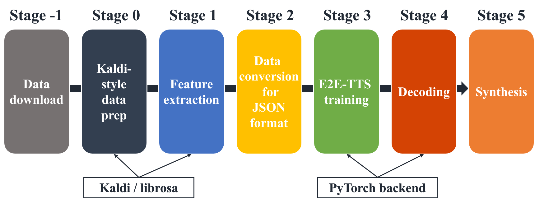
- stage -1: Download data if the data is available online.
- stage 0: Prepare data to make kaldi-stype data directory.
- stage 1: Extract feature vector, calculate statistics, and normalize.
- stage 2: Prepare a dictionary and make json files for training.
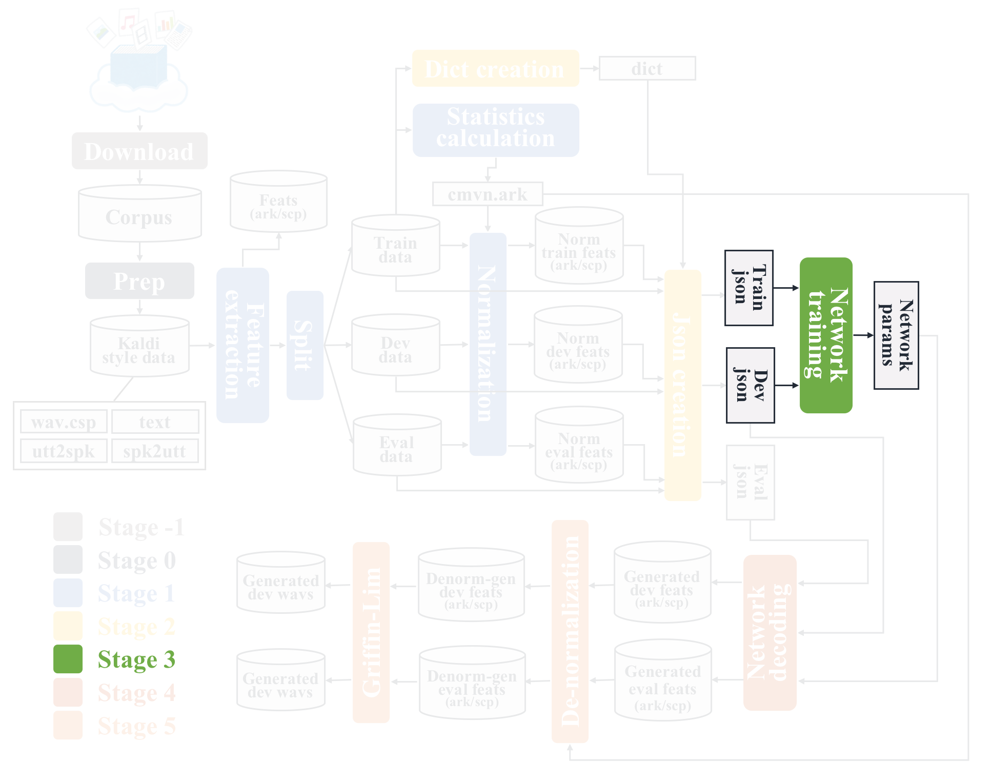
- stage 3: Train the E2E-TTS network.
- stage 4: Decode mel-spectrogram using the trained network.
- stage 5: Generate a waveform using Griffin-Lim.
From stage -1 to 2 are the same as the ASR recipe.
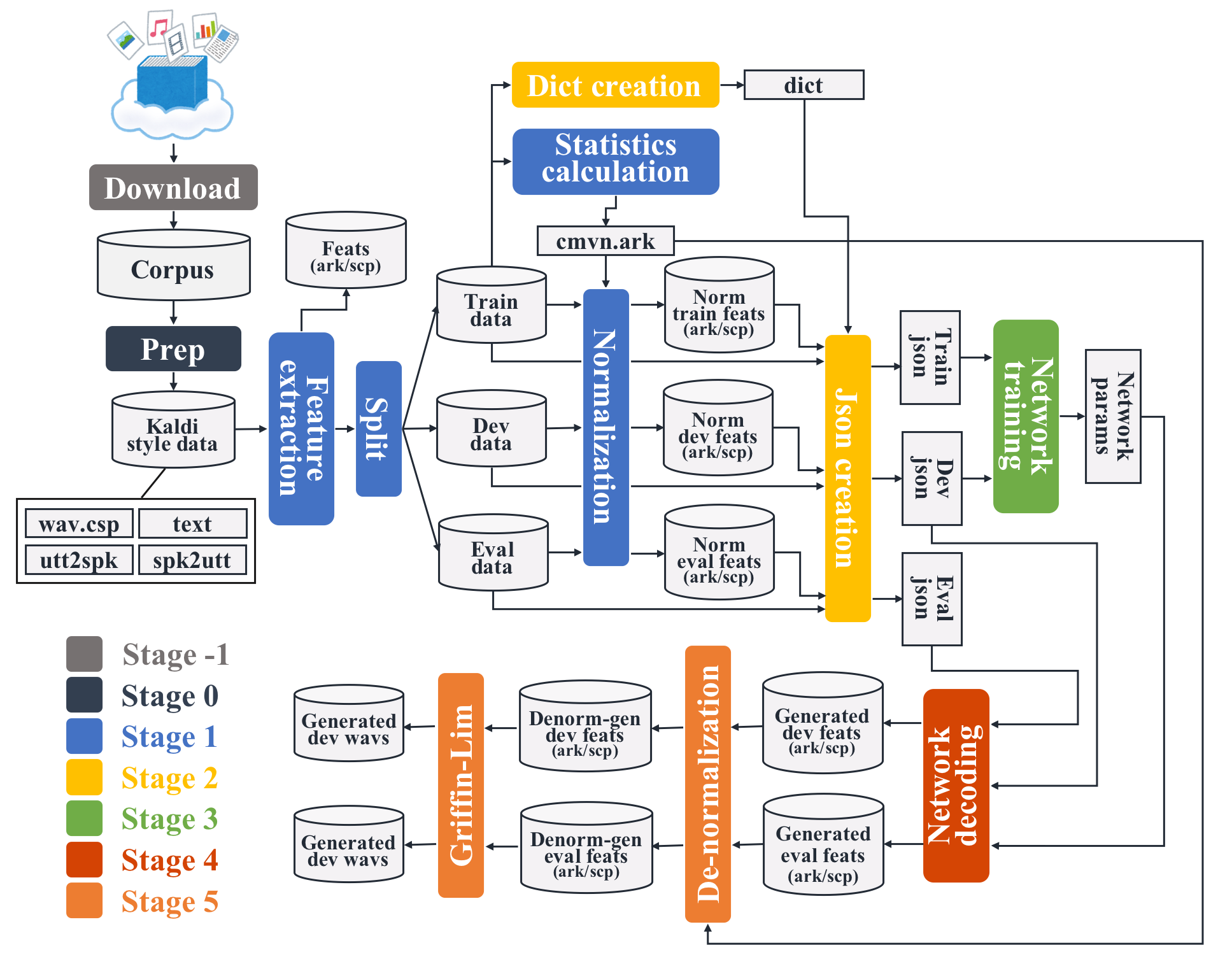
Detail overview

# run stage -1 and then stop
!./run.sh --stage -1 --stop_stage -1
downloads directory is created, which containing downloaded an4 dataset.
!tree -L 2 downloads

# run stage 0 and then stop
!./run.sh --stage 0 --stop_stage 0
Two kaldi-style data directories are created:
data/train: data directory of training setdata/test: data directory of evaluation set
!tree -L 2 data
wav.scp:
- Each line has
<utt_id> <wavfile_path or command pipe> <utt_id>must be unique
text:
- Each line has
<utt_id> <transcription> - Assume that
<transcription>is cleaned
utt2spk:
- Each line has
<utt_id> <speaker_id>
spk2utt:
- Each line has
<speaker_id> <utt_id> ... <utt_id> - Can be automatically created from
utt2spk
In the ESPnet, speaker information is not used for any processing.
Therefore, utt2spk and spk2utt can be a dummy.
!head -n 3 data/train/*
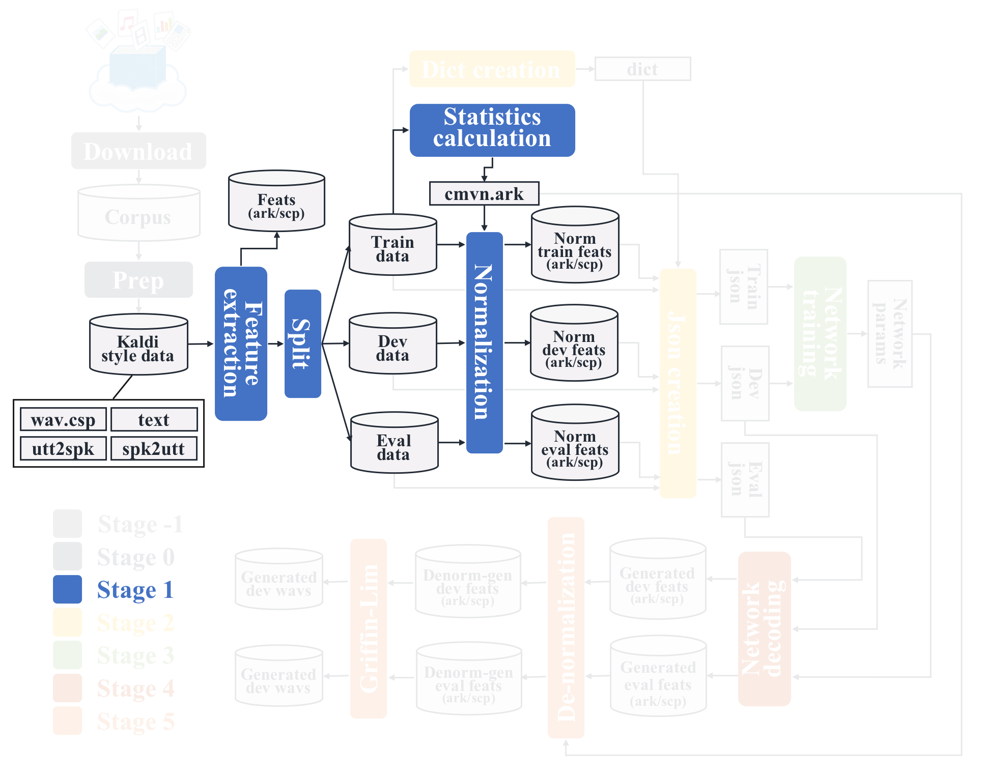
Stage 1: Feature extration
This stage performs feature extraction, statistics calculation and normalization.
# hyperparameters related to stage 1
!head -n 28 run.sh | tail -n 8
# run stage 1 with default settings
!./run.sh --stage 1 --stop_stage 1 --nj 4
Raw filterbanks are saved in fbank/ directory with ark/scp format.
.ark: binary file of feature vector.scp: list of the correspondance b/w<utt_id>and<path_in_ark>.
Since feature extraction can be performed for split small sets in parallel, raw_fbank is split into raw_fbank_*.{1..4}.{scp,ark}.
!tree -L 2 fbank
!head -n 3 fbank/raw_fbank_train.1.scp
These files can be loaded in python via a great tool kaldiio as follows:
import kaldiio
import matplotlib.pyplot as plt

# load scp file
scp_dict = kaldiio.load_scp("fbank/raw_fbank_train.1.scp")
for key in scp_dict:
    plt.imshow(scp_dict[key].T[::-1])
    plt.title(key)
    plt.colorbar()
    plt.show()
    break

# load ark file
ark_generator = kaldiio.load_ark("fbank/raw_fbank_train.1.ark")
for key, array in ark_generator:
    plt.imshow(array.T[::-1])
    plt.title(key)
    plt.colorbar()
    plt.show()
    break
Some files are added in data/train:
feats.scp: concatenated scp file offbank/raw_fbank_train.{1..4}.scp.utt2num_frames: Each line has<utt_id> <number_of_frames>.
!tree data/train
!head -n 3 data/train/*
data/train/ directory is split into two directories:
data/train_nodev/: data directory for trainingdata/train_dev/: data directory for validation
!tree data/train_*
cmvn.ark is saved in data/train_nodev, which is the statistics file.
(cepstral mean variance normalization: cmvn)
This file also can be loaded in python via kaldiio.
!tree data/train_nodev
Normalized features for train, dev, and eval sets are dumped in
dump/{train_nodev,train_dev,test}/*.{ark,scp}.
These ark and scp can be loaded as the same as the above procedure.
!tree dump/*
Stage 2: Dictionary and json preparation
This stage creates char dict and integrate files into a single json file.

# run stage 2 and then stop
!./run.sh --stage 2 --stop_stage 2
- Dictionary file is created in
data/lang_1char/. - Dictionary file consists of
<token><token index>.<token index>starts from 1 because 0 is used as padding index.
!tree data/lang_1char
!cat data/lang_1char/train_nodev_units.txt
Three json files are created for train, dev, and eval sets as
dump/{train_nodev,train_dev,test}/data.json.
!tree dump -L 2
Each json file contains all of the information in the data directory.
shape: Shape of the input or output sequence.text: Original transcription.token: Token sequence of the transcription.tokenidToken id sequence converted withdictof the transcription
!head -n 27 dump/train_nodev/data.json
Now ready to start training!
Training setting can be specified by train_config.
# check hyperparmeters in run.sh
!head -n 31 run.sh | tail -n 2
Training configuration is written in .yaml format file.
Let us check the default configuration conf/train_pytroch_tacotron2.yaml.
!cat conf/train_pytorch_tacotron2.yaml
Let's change the hyperparameters.
# load configuration yaml
import yaml
with open("conf/train_pytorch_tacotron2.yaml") as f:
    params = yaml.load(f, Loader=yaml.Loader)

# change hyperparameters by yourself!
params.update({
    "embed-dim": 16,
    "elayers": 1,
    "eunits": 16,
    "econv-layers": 1,
    "econv-chans": 16,
    "econv-filts": 5,
    "dlayers": 1,
    "dunits": 16,
    "prenet-layers": 1,
    "prenet-units": 16,
    "postnet-layers": 1,
    "postnet-chans": 16,
    "postnet-filts": 5,
    "adim": 16,
    "aconv-chans": 16,
    "aconv-filts": 5,
    "reduction-factor": 5,
    "batch-size": 128,
    "epochs": 5,
    "report-interval-iters": 10,
})

# save
with open("conf/train_pytorch_tacotron2_mini.yaml", "w") as f:
    yaml.dump(params, f, Dumper=yaml.Dumper)

# check modified version
!cat conf/train_pytorch_tacotron2_mini.yaml
Also, we provide transformer and fastspeech configs.
!cat ../../ljspeech/tts1/conf/tuning/train_pytorch_transformer.v1.yaml
!cat ../../ljspeech/tts1/conf/tuning/train_fastspeech.v2.yaml
We can easily switch the model to be trained by only changing --train_config.
(NOTE: FastSpeech needs a teacher model, pretrained Transformer)
Let's train the network.
You can specify the config file via --train_config option.
It takes several minutes.
# use modified configuration file as train config
!./run.sh --stage 3 --stop_stage 3 --train_config conf/train_pytorch_tacotron2_mini.yaml --verbose 1
You can see the training log in exp/train_*/train.log.
!cat exp/train_nodev_pytorch_train_pytorch_tacotron2_mini/train.log
The models are saved in exp/train_*/results/ directory.
exp/train_*/results/model.loss.best: contains only the model parameters.exp/train_*/results/snapshot.ep.*: contains the model parameters, optimizer states, and iterator states.
!tree -L 1 exp/train_nodev_pytorch_train_pytorch_tacotron2_mini/results
exp/train_*/results/*.png are the figures of training curve.
Let us check them.
from IPython.display import Image, display_png
print("all loss curve")
display_png(Image("exp/train_nodev_pytorch_train_pytorch_tacotron2_mini/results/all_loss.png", width=500))
print("l1 loss curve")
display_png(Image("exp/train_nodev_pytorch_train_pytorch_tacotron2_mini/results/l1_loss.png", width=500))
print("mse loss curve")
display_png(Image("exp/train_nodev_pytorch_train_pytorch_tacotron2_mini/results/mse_loss.png", width=500))
print("bce loss curve")
display_png(Image("exp/train_nodev_pytorch_train_pytorch_tacotron2_mini/results/bce_loss.png", width=500))
exp/train_*/results/att_ws/*.png are the figures of attention weights in each epoch.
In the case of E2E-TTS, it is very important to check that they are diagonal.
print("Attention weights of initial epoch")
display_png(Image("exp/train_nodev_pytorch_train_pytorch_tacotron2_mini/results/att_ws/fash-cen1-b.ep.1.png", width=500))
Example of a good diagonal attention weights:

Also, we support tensorboard.
You can see the training log through tensorboard.
# only available in colab
%load_ext tensorboard
%tensorboard --logdir tensorboard/train_nodev_pytorch_train_pytorch_tacotron2_mini/

Decoding parameters can be specified by --decode_config.
!head -n 32 run.sh | tail -n 1
Decoding configuration in written in .yaml format file.
Let us check the default configuration conf/decode.yaml.
!cat conf/decode.yaml
Let us modify to stop the generation in early steps.
# load configuration yaml
import yaml
with open("conf/decode.yaml") as f:
    params = yaml.load(f, Loader=yaml.Loader)

# change hyperparameters by yourself!
params.update({
    "maxlenratio": 1.0,
})

# save
with open("conf/decode_mini.yaml", "w") as f:
    yaml.dump(params, f, Dumper=yaml.Dumper)

# check modified version
!cat conf/decode_mini.yaml
# run stage 4 and then stop
!./run.sh --stage 4 --stop_stage 4 --nj 2 --verbose 1 \
    --train_config conf/train_pytorch_tacotron2_mini.yaml \
    --decode_config conf/decode_mini.yaml
Generated features are saved as ark/scp format.
Also figures of attention weights and stop probabilities are saved as {att_ws/probs}/*.png.
!tree -L 2 exp/train_nodev_pytorch_train_pytorch_tacotron2_mini/outputs_model.loss.best_decode*

# run stage 5 and then stop
!./run.sh --stage 5 --stop_stage 5 --nj 2 \
    --train_config conf/train_pytorch_tacotron2_mini.yaml \
    --decode_config conf/decode_mini.yaml \
    --griffin_lim_iters 4
Please run stage 5.
Generated wav files are saved in
exp/train_nodev_pytorch_*/outputs_model.loss.best_*_denorm/{train_dev,test}/wav/
!tree -L 2 exp/train_nodev_pytorch_train_pytorch_tacotron2_mini/*_denorm
Now you finish building your own E2E-TTS model!
But unfortunately, this model cannot generate a good speech.
Let us listen to the samples in demo HP to check the quality.
https://espnet.github.io/espnet-tts-sample/
3. Demonstration of the use of TTS pretrained models
We provide pretrained TTS models and these are easy to use with espnet/utils/synth_wav.sh.
# move on directory
os.chdir("../../librispeech/asr1")
!pwd
Let us check the usage of espnet/utils/synth_wav.sh.
It will automatically downloads pretrained model from online, you do not need to prepare anything.
!../../../utils/synth_wav.sh --help
Let us generate your own text with pretrained models!
# generate your sentence!
!rm -rf decode/example
print("Please input your favorite sentence!")
text = input()
text = text.upper()
with open("example.txt", "w") as f:
    f.write(text + "\n")

# you can change here to select the pretrained model
!../../../utils/synth_wav.sh --stop_stage 3 --models ljspeech.fastspeech.v1 example.txt
# !../../../utils/synth_wav.sh --stop_stage 3 --models ljspeech.tacotron2.v3 example.txt
# !../../../utils/synth_wav.sh --stop_stage 3 --models ljspeech.transformer.v1 example.txt

# check generated audio
from IPython.display import display, Audio, Image, display_png
display(Audio("decode/example/wav/example_1.wav"))
!sox decode/example/wav/example_1.wav -n rate 22050 spectrogram
display_png(Image("spectrogram.png", width=750))

# check attention and probs
if os.path.exists("decode/example/outputs/att_ws/example_1_att_ws.png"):
    display_png(Image("decode/example/outputs/att_ws/example_1_att_ws.png", width=1000))
    display_png(Image("decode/example/outputs/probs/example_1_prob.png", width=500))
Also you can try the neural vocoder.
# generate your sentence!
!rm -rf decode/example_short
print("Please input your favorite sentence!")
text = input()
text = text.upper()
with open("example_short.txt", "w") as f:
    f.write(text + "\n")

# extend stop_stage
!../../../utils/synth_wav.sh --stop_stage 4 --models ljspeech.tacotron2.v3 example_short.txt

# check generated audio
display(Audio("decode/example_short/wav/example_short_1.wav"))
display(Audio("decode/example_short/wav_wnv/example_short_1_gen.wav"))
4. Demonstration of the use of ASR pretrained models
ESPnet also provides the espnet/utils/recog_wav.sh to use pretrained ASR models.
Let us recognize the generated speech!
!../../../utils/recog_wav.sh --help
# downsample to 16 kHz for ASR model
!sox decode/example/wav/example_1.wav -b 16 decode/example/wav/example_1_16k.wav rate 16k pad 0.1 pad 0 0.1

# make decode config
import yaml
with open("conf/decode_sample.yaml", "w") as f:
    yaml.dump({
        "batchsize": 0,
        "beam-size": 5,
        "ctc-weight": 0.4,
        "lm-weight": 0.6,
        "maxlenratio": 0.0,
        "minlenratio": 0.0,
        "penalty": 0.0,
    }, f, Dumper=yaml.Dumper)

# let's recognize generated speech
!../../../utils/recog_wav.sh --models librispeech.transformer.v1 \
    --decode_config conf/decode_sample.yaml \
    decode/example/wav/example_1_16k.wav
Conclusion
- Can build E2E-TTS models with unified-design recipe
- Can try various models by just changing the yaml file
Through ESPnet, you can build / use E2E-TTS and E2E-ASR in the same manner!
Thank you for your attention!