using AIBECS
using PyPlot, PyCall
using LinearAlgebra
AIBECS.jl
The ideal tool for exploring global marine biogeochemical cycles
Algebraic Implicit Biogeochemical Elemental Cycling System
Check it on GitHub (look for AIBECS.jl)

with François Primeau and J. Keith Moore
Outline
- Motivation and concept
- Example 1: Radiocarbon
- Toy model circulation
- OCIM1
- Example 2: Phosphorus cycle
- AIBECS ecosystem
Motivation: Starting from the AWESOME OCIM
The AWESOME OCIM (for A Working Environment for Simulating Ocean Movement and Elemental cycling in an Ocean Circulation Inverse Model framework) by Seth John (USC)
Features: GUI, simple to use, fast, and good circulation
(thanks to the OCIM1 by Tim DeVries (UCSB))
Motivation: comes the AIBECS
Features (at present)
- simple to use
- fast
- Julia instead of MATLAB (free, open-source, better performance, and better syntax)
- nonlinear systems
- multiple tracers
- Other circulations (not just the OCIM)
- Parameter estimation/optimization and Senstivity analysis (shameless plug: F-1 algorithm seminar tomorrow at the School of Mathematics)

AIBECS Concept: a simple interface
To build a BGC model with the AIBECS, you just need to
1. Specify the local sources and sinks
2. Chose the ocean circulation
(3. Specify the particle transport, if any)
AIBECS concept: Vectorization
The 3D ocean grid is rearranged
into a 1D column vector.
And linear operators are represented by matrices.
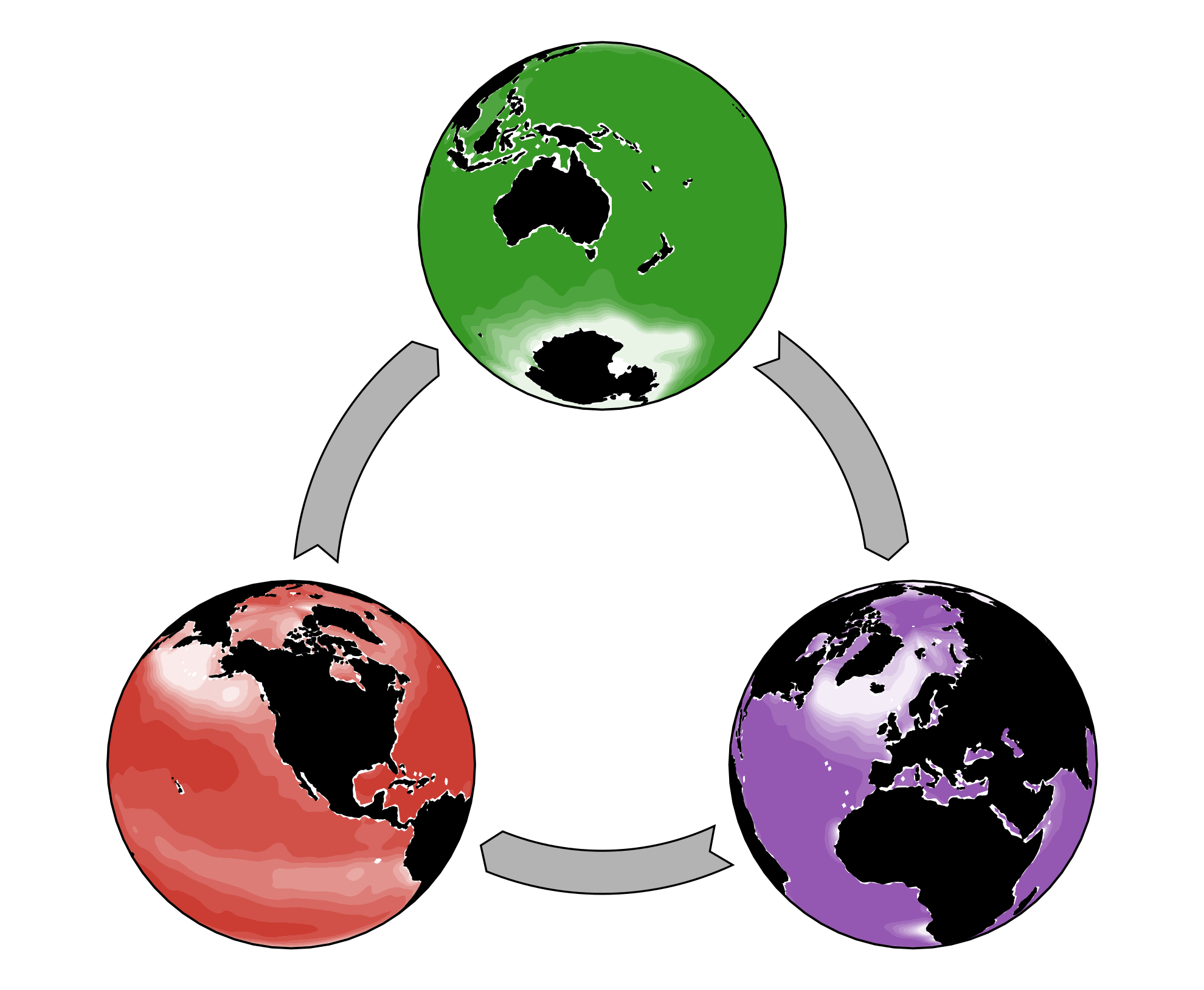
Example 1: Radiocarbon, a tracer for water age

Image credit: Luke Skinner, University of Cambridge
Tracer equation: transport + sources and sinks
The Tracer equation ($x=$ Radiocarbon concentration)
$$\frac{\partial x}{\partial t} + \color{RoyalBlue}{\nabla \cdot \left[ \boldsymbol{u} - \mathbf{K} \cdot \nabla \right]} x = \color{ForestGreen}{\underbrace{\Lambda(x)}_{\textrm{air–sea exchange}} - \underbrace{x / \tau}_{\textrm{radioactive decay}}}$$becomes
$$\frac{\partial \boldsymbol{x}}{\partial t} + \color{RoyalBlue}{\mathbf{T}} \, \boldsymbol{x} = \color{ForestGreen}{\mathbf{\Lambda}(\boldsymbol{x}) - \boldsymbol{x} / \tau}.$$with the transport matrix
Translating to AIBECS Code is easy
To use AIBECS, we must recast each tracer equation,
$$\frac{\partial \boldsymbol{x}}{\partial t} + \color{RoyalBlue}{\mathbf{T}} \, \boldsymbol{x} = \color{ForestGreen}{\mathbf{\Lambda}(\boldsymbol{x}) - \boldsymbol{x} / \tau}$$here, into the generic form:
$$\frac{\partial \boldsymbol{x}}{\partial t} + \color{RoyalBlue}{\mathbf{T}(\boldsymbol{p})} \, \boldsymbol{x} = \color{ForestGreen}{\boldsymbol{G}(\boldsymbol{x}, \boldsymbol{p})}$$where $\boldsymbol{p} =$ vector of model parameters
Circulation 1: The 2×2×2 Primeau model
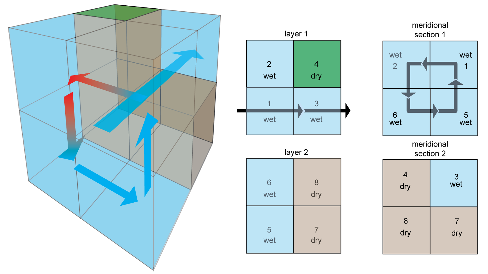
- ACC: Antarctic Circumpolar Current
- MOC: Meridional Overturning Circulation
- High-latitude mixing
(Credit: François Primeau, and Louis Primeau for the image)
Load the circulation via load:
wet3D, grd, T = Primeau_2x2x2.load();
Creating François Primeau's 2x2x2 model ✔

wet3D is the mask of "wet" points
wet3D
2×2×2 BitArray{3}:
[:, :, 1] =
 true   true
 true  false

[:, :, 2] =
 true  false
 true  false
grd is the grid of the circulation
grd
OceanGrid of size 2×2×2 (lat×lon×depth)
We can check the depth of the boxes arranged in 3D
grd.depth_3D
2×2×2 Array{Quantity{Float64,𝐋,Unitful.FreeUnits{(m,),𝐋,nothing}},3}:
[:, :, 1] =
 100.0 m  100.0 m
 100.0 m  100.0 m

[:, :, 2] =
 1950.0 m  1950.0 m
 1950.0 m  1950.0 m

T
5×5 SparseMatrixCSC{Float64,Int64} with 12 stored entries:
  [1, 1]  =  4.50923e-9
  [2, 1]  =  -5.88161e-10
  [3, 1]  =  -3.92107e-9
  [2, 2]  =  9.80268e-10
  [5, 2]  =  -5.60153e-11
  [1, 3]  =  -3.92107e-9
  [3, 3]  =  3.92107e-9
  [1, 4]  =  -5.88161e-10
  [4, 4]  =  3.36092e-11
  [2, 5]  =  -3.92107e-10
  [4, 5]  =  -3.36092e-11
  [5, 5]  =  5.60153e-11
A sparse matrix is indexed by its non-zero values,
but we can check it out in full using Matrix:
Matrix(T)
5×5 Array{Float64,2}:
  4.50923e-9    0.0          -3.92107e-9  -5.88161e-10   0.0
 -5.88161e-10   9.80268e-10   0.0          0.0          -3.92107e-10
 -3.92107e-9    0.0           3.92107e-9   0.0           0.0
  0.0           0.0           0.0          3.36092e-11  -3.36092e-11
  0.0          -5.60153e-11   0.0          0.0           5.60153e-11
Sources and sinks
Tracer equation reminder:
$$\frac{\partial \boldsymbol{x}}{\partial t} + \mathbf{T}(\boldsymbol{p}) \, \boldsymbol{x} = \boldsymbol{G}(\boldsymbol{x}, \boldsymbol{p})$$Let's write $\boldsymbol{G}(\boldsymbol{x}, \boldsymbol{p}) = \mathbf{\Lambda}(\boldsymbol{x}) - \boldsymbol{x} / \tau$
G(x,p) = Λ(x,p) - x / p.τ
G (generic function with 1 method)
Air–sea gas exchange
And define the air–sea gas exchange $\mathbf{\Lambda}(\boldsymbol{x}) = \frac{\lambda}{h} (R_\mathsf{atm} - \boldsymbol{x})$ at the surface with a piston velocity $\lambda$ over the top layer of height $h$
function Λ(x,p)
    λ, h, Ratm = p.λ, p.h, p.Ratm
    return @. λ / h * (Ratm - x) * (z == z₀)
end
Λ (generic function with 1 method)
Define z the depths in vector form.
(iwet converts from 3D to 1D)
iwet = findall(wet3D)
z = grd.depth_3D[iwet]
5-element Array{Quantity{Float64,𝐋,Unitful.FreeUnits{(m,),𝐋,nothing}},1}:
  100.0 m
  100.0 m
  100.0 m
 1950.0 m
 1950.0 m
Define z₀ the depth of the top layer
z₀ = z[1]
100.0 m
So that z .== z₀ is true at the surface layer
z .== z₀
5-element BitArray{1}:
  true
  true
  true
 false
 false
Model parameters
First, create a table of parameters using the AIBECS API
t = empty_parameter_table()
add_parameter!(t,    :τ, 5730u"yr" / log(2)) # radioactive decay e-folding timescale
add_parameter!(t,    :λ,   50u"m" / 10u"yr") # piston velocity
add_parameter!(t,    :h,      grd.δdepth[1]) # top layer height
add_parameter!(t, :Ratm,      1.0u"mol/m^3") # atmospheric concentration
t
| symbol | value | unit | printunit | mean_obs | variance_obs | optimizable | description | |
|---|---|---|---|---|---|---|---|---|
| Symbol | Float64 | Unitful… | Unitful… | Float64 | Float64 | Bool | String | |
| 1 | τ | 2.60875e11 | s | yr | NaN | NaN | false | |
| 2 | λ | 1.5844e-7 | m s^-1 | m yr^-1 | NaN | NaN | false | |
| 3 | h | 200.0 | m | m | NaN | NaN | false | |
| 4 | Ratm | 1.0 | mol m^-3 | mol m^-3 | NaN | NaN | false |
Then, chose a name for the parameters (here C14_parameters), and create the vector p:
initialize_Parameters_type(t, "C14_parameters")
p = C14_parameters()
     τ = 8.27e+03 [yr] (fixed)
     λ = 5.00e+00 [m yr⁻¹] (fixed)
     h = 2.00e+02 [m] (fixed)
  Ratm = 1.00e+00 [mol m⁻³] (fixed)
C14_parameters{Float64}
Note p has units!
In AIBECS, you give your parameters units and they are automatically converted to SI units under the hood.
(And they are converted back for pretty printing!)
State function (and Jacobian)
Rearrange the tracer equation into
$$\frac{\partial \boldsymbol{x}}{\partial t} = \boldsymbol{G}(\boldsymbol{x}, \boldsymbol{p}) - \mathbf{T}(\boldsymbol{p}) \, \boldsymbol{x} = \color{Brown}{\boldsymbol{F}(\boldsymbol{x}, \boldsymbol{p})}$$We generate F and ∇ₓF via
F, ∇ₓF = state_function_and_Jacobian(p -> T, G) ;
The state function F(x,p)
Let's try F on a random state vector x
x = 0.5p.Ratm * ones(5)
F(x,p)
5-element Array{Float64,1}:
  3.941844738773137e-10
  3.941844738773139e-10
  3.941844738773139e-10
 -1.916623798048004e-12
 -1.916623798048004e-12
The Jacobian ∇ₓF
The Jacobian matrix is $\nabla_{\boldsymbol{x}}\boldsymbol{F}(\boldsymbol{x},\boldsymbol{p}) = \left[\frac{\partial F_i}{\partial x_j}\right]_{i,j}$, is useful for
- implicit time-steps
- solving the steady-state system
- optimization / uncertainty analysis
With AIBECS, the Jacobian is computed automatically for you under the hood... using dual numbers!
(Come to my Applied seminar tomorrow for more on dual numbers and... hyperdual numbers!)
Let's try ∇ₓF at x:
Matrix(∇ₓF(x,p))
5×5 Array{Float64,2}:
 -5.30527e-9    0.0           3.92107e-9   5.88161e-10   0.0
  5.88161e-10  -1.7763e-9     0.0          0.0           3.92107e-10
  3.92107e-9    0.0          -4.71711e-9   0.0           0.0
  0.0           0.0           0.0         -3.74424e-11   3.36092e-11
  0.0           5.60153e-11   0.0          0.0          -5.98486e-11
Time stepping
AIBECS provides schemes for time-stepping
- Euler forward
- Euler backward
- Crank-Nicolson
- Crank-Nicolson leap-frog
Let's track the evolution of x through time
Define a function to apply the time steps n times for a time span of Δt starting from x₀
function time_steps(x₀, Δt, n, F, ∇ₓF)
    x_hist = [x₀]
    δt = Δt / n
    for i in 1:n
        push!(x_hist, AIBECS.crank_nicolson_step(last(x_hist), p, δt, F, ∇ₓF))
    end
    return reduce(hcat, x_hist), 0:δt:Δt
end
time_steps (generic function with 1 method)
Let's run the model for 5000 years starting with x = 1 everywhere:
Δt = 5000u"yr" |> u"s" |> ustrip
x₀ = p.Ratm * ones(5)
x_hist, t_hist = time_steps(x₀, Δt, 1000, F, ∇ₓF)
([1.0 0.99943 … 0.940489 0.940485; 1.0 0.99943 … 0.954752 0.95475; … ; 1.0 0.999395 … 0.804853 0.804839; 1.0 0.999395 … 0.894027 0.894023], 0.0:1.57788e8:1.57788e11)
Plotting the output is easy
The radiocarbon age, C14age, is given by $\log(R_{\mathrm{atm}}/\boldsymbol{x}) \tau$ because $\boldsymbol{x}\sim R_{\mathrm{atm}} \exp(-t/\tau)$
Let's plot its evolution with time:
C14age_hist = log.(p.Ratm ./ x_hist) * (p.τ * u"s" |> u"yr" |> ustrip)
PyPlot.figure(figsize=(8,4))
PyPlot.plot(t_hist .* 1u"s" .|> u"yr" .|> ustrip, C14age_hist')
PyPlot.xlabel("simulation time (years)")
PyPlot.ylabel("¹⁴C age (years)")
PyPlot.legend("box " .* string.(findall(vec(wet3D))))
PyPlot.title("Simulation of the evolution of ¹⁴C age with Crank-Nicolson time steps")

PyObject Text(0.5, 1, 'Simulation of the evolution of ¹⁴C age with Crank-Nicolson time steps')
Solve directly for the steady state
Instead, we can directly solve for the steady-state, $\boldsymbol{s}$,
(using CTKAlg(), a quasi-Newton root-finding algorithm from C. T. Kelley)
i.e., such that $\boldsymbol{F}(\boldsymbol{s},\boldsymbol{p}) = 0$:
prob = SteadyStateProblem(F, ∇ₓF, x, p)
s = solve(prob, CTKAlg()).u
5-element Array{Float64,1}:
 0.9395557449765635
 0.9542341322419017
 0.9489433863241392
 0.8016816657976089
 0.8931162915594038
gives the age
log.(p.Ratm ./ s) * (p.τ * u"s" |> u"yr")
5-element Array{Quantity{Float64,𝐓,Unitful.FreeUnits{(yr,),𝐓,nothing}},1}:
   515.409683042318 yr
  387.2609241614547 yr
  433.2228144719123 yr
 1827.2890596434506 yr
  934.4487196556533 yr
Circulation 2: OCIM1
The Ocean Circulation Inverse Model (OCIM) version 1 is loaded via
wet3D, grd, T = OCIM1.load() ;
Loading OCIM1 ✔
┌ Info: You are about to use OCIM1 model.
│ If you use it for research, please cite:
│
│ - DeVries, T., 2014: The oceanic anthropogenic CO2 sink: Storage, air‐sea fluxes, and transports over the industrial era, Global Biogeochem. Cycles, 28, 631–647, doi:10.1002/2013GB004739.
│ - DeVries, T. and F. Primeau, 2011: Dynamically and Observationally Constrained Estimates of Water-Mass Distributions and Ages in the Global Ocean. J. Phys. Oceanogr., 41, 2381–2401, doi:10.1175/JPO-D-10-05011.1
│
│ You can find the corresponding BibTeX entries in the CITATION.bib file
│ at the root of the AIBECS.jl package repository.
│ (Look for the "DeVries_Primeau_2011" and "DeVries_2014" keys.)
└ @ AIBECS.OCIM1 /Users/benoitpasquier/.julia/dev/AIBECS/src/OCIM1.jl:53
Redefine F and ∇ₓF for the new T:
F, ∇ₓF = state_function_and_Jacobian(p -> T, G) ;
Redefine iwet and x for the new grid size
iwet = findall(wet3D)
x = p.Ratm * ones(length(iwet))
200160-element Array{Float64,1}:
 1.0
 1.0
 1.0
 1.0
 1.0
 1.0
 1.0
 1.0
 1.0
 1.0
 1.0
 1.0
 1.0
 ⋮
 1.0
 1.0
 1.0
 1.0
 1.0
 1.0
 1.0
 1.0
 1.0
 1.0
 1.0
 1.0
Redefine h, z₀, and z for the new grid
p.h = grd.δdepth[1] |> upreferred |> ustrip
z = grd.depth_3D[iwet]
z₀ = z[1]
18.0675569520817 m
Solve for the steady-state of radio carbon and convert to age
prob = SteadyStateProblem(F, ∇ₓF, x, p)
s = solve(prob, CTKAlg()).u
C14age = log.(p.Ratm ./ s) * p.τ * u"s" .|> u"yr"
200160-element Array{Quantity{Float64,𝐓,Unitful.FreeUnits{(yr,),𝐓,nothing}},1}:
 1364.7245332141904 yr
 1376.8840164693377 yr
  1395.880072599861 yr
 1383.0420964666034 yr
 1300.9081458733074 yr
 1277.2701118588532 yr
 1304.3367306286561 yr
  1288.118038954236 yr
  1247.320711595564 yr
 1190.1083953526847 yr
  1138.219050291774 yr
 1101.7243454552279 yr
 1049.2576207122263 yr
                     ⋮
 1117.4712399943664 yr
  1114.907399656483 yr
 1120.6568745437007 yr
 1114.5505967309834 yr
 1107.5809181397601 yr
 1123.3995401256584 yr
 1119.1390345237028 yr
  1111.881056087309 yr
 1097.5315397930838 yr
 1118.1355949317388 yr
  1114.114095931889 yr
 1109.1001449651774 yr
And plot horizontal slices using GR and Interact:
lon, lat = grd.lon |> ustrip, grd.lat |> ustrip
ccrs = pyimport("cartopy.crs")
cfeature = pyimport("cartopy.feature")
lon_cyc = [lon; 360+lon[1]]
function horizontal_slice(x, iz, levels, title, unit)
    figure(figsize=(12,5))
    x_3D = fill(NaN, size(grd))
    x_3D[iwet] .= x .|> ustrip
    x_3D_cyc = cat(x_3D, x_3D[:,[1],:], dims=2)
    ax = PyPlot.subplot(projection = ccrs.EqualEarth(central_longitude=-155.0))
    ax.add_feature(cfeature.COASTLINE, edgecolor="#000000") # black coast lines
    ax.add_feature(cfeature.LAND, facecolor="#CCCCCC")      # gray land
    plt = PyPlot.contourf(lon_cyc, lat, x_3D_cyc[:,:,iz], levels=levels, transform=ccrs.PlateCarree(), zorder=-1, extend="both")
    plt2 = PyPlot.contour(plt, lon_cyc, lat, x_3D_cyc[:,:,iz], levels=plt.levels[1:5:end], transform=ccrs.PlateCarree(), zorder=0, extend="both", colors="k")
    ax.clabel(plt2, fmt="%2.1f", colors="k", fontsize=14)
    cbar = PyPlot.colorbar(plt, orientation="vertical", extend="both", ticks=plt2.levels)
    cbar.add_lines(plt2)
    cbar.ax.tick_params(labelsize=14)
    cbar.set_label(label=unit, fontsize=16)
    PyPlot.title(string(title, " at $(AIBECS.round(grd.depth[iz])) depth"), fontsize=20)
end
horizontal_slice(C14age, 12, 0:100:2400, "14C age using the OCIM1 circulation", "yr")

PyObject Text(0.5, 1, '14C age using the OCIM1 circulation at 919.0 m depth')
Or zonal slices:
depth = grd.depth .|> ustrip
function zonal_slice(x, ix, levels, title, unit)
    figure(figsize=(12,5))
    x_3D = fill(NaN, size(grd))
    x_3D[iwet] .= x .|> ustrip
    ax = subplot()
    plt = PyPlot.contourf(lat, depth, x_3D[:,ix,:]', levels=levels, extend="both")
    ax.invert_yaxis()
    plt2 = PyPlot.contour(plt, lat, depth, x_3D[:,ix,:]', levels=plt.levels[1:5:end], extend="both", colors="k")
    ax.clabel(plt2, fmt="%2.1f", colors="k", fontsize=14)
    cbar = PyPlot.colorbar(plt, orientation="vertical", extend="both", ticks=plt2.levels)
    cbar.add_lines(plt2)
    cbar.ax.tick_params(labelsize=14)
    cbar.set_label(label=unit, fontsize=16)
    PyPlot.title(string(title, " at $(AIBECS.round(grd.lon[ix])) longitude"), fontsize=20)
end
zonal_slice(C14age, 165, 0:100:2400, "14C age [yr] using the OCIM1 circulation", "yr")

PyObject Text(0.5, 1, '14C age [yr] using the OCIM1 circulation at 329.0° longitude')

Example 2: A phosphorus cycle
Dissolved inorganic phosphrous (DIP)
(transported by the ocean circulation)
and particulate organic phosphrous (POP)
(transported by sinking particles)
Ocean circulation
For DIP, the advective–eddy-diffusive transport operator, $\nabla \cdot (\boldsymbol{u} + \mathbf{K}\cdot\nabla)$, is converted into the matrix T:
T_DIP(p) = T
T_DIP (generic function with 1 method)
Sinking particles
For POP, the particle flux divergence (PFD) operator, $\nabla \cdot \boldsymbol{w}$, is created via buildPFD:
T_POP(p) = buildPFD(grd, wet3D, sinking_speed = w(p))
T_POP (generic function with 1 method)
The settling velocity, w(p), is assumed linearly increasing with depth z to yield a "Martin curve profile"
w(p) = p.w₀ .+ p.w′ * (z .|> ustrip)
w (generic function with 1 method)
relu(x) = (x .≥ 0) .* x
zₑ = 80u"m"    # depth of the euphotic zone
function uptake(DIP, p)
    τ, k = p.τ, p.k
    DIP⁺ = relu(DIP)
    return 1/τ * DIP⁺.^2 ./ (DIP⁺ .+ k) .* (z .≤ zₑ)
end
uptake (generic function with 1 method)
remineralization(POP, p) = p.κ * POP
remineralization (generic function with 1 method)
geores(x, p) = (p.xgeo .- x) / p.τgeo
geores (generic function with 1 method)
G_DIP(DIP, POP, p) = -uptake(DIP, p) + remineralization(POP, p) + geores(DIP, p)
G_POP(DIP, POP, p) =  uptake(DIP, p) - remineralization(POP, p)
G_POP (generic function with 1 method)
Parameters
t = empty_parameter_table()    # empty table of parameters
add_parameter!(t, :xgeo, 2.12u"mmol/m^3")
add_parameter!(t, :τgeo, 1.0u"Myr")
add_parameter!(t, :k, 6.62u"μmol/m^3")
add_parameter!(t, :w₀, 0.64u"m/d")
add_parameter!(t, :w′, 0.13u"1/d")
add_parameter!(t, :κ, 0.19u"1/d")
add_parameter!(t, :τ, 236.52u"d")
initialize_Parameters_type(t, "Pcycle_Parameters")   # Generate the parameter type
p = Pcycle_Parameters()
  xgeo = 2.12e+00 [mmol m⁻³] (fixed)
  τgeo = 1.00e+00 [Myr] (fixed)
     k = 6.62e+00 [μmol m⁻³] (fixed)
    w₀ = 6.40e-01 [m d⁻¹] (fixed)
    w′ = 1.30e-01 [d⁻¹] (fixed)
     κ = 1.90e-01 [d⁻¹] (fixed)
     τ = 2.37e+02 [d] (fixed)
Pcycle_Parameters{Float64}
State function F and Jacobian ∇ₓF
nb = length(iwet); x = ones(2nb)
F, ∇ₓF = state_function_and_Jacobian((T_DIP,T_POP), (G_DIP,G_POP), nb) ;
Solve the steady-state PDE system
prob = SteadyStateProblem(F, ∇ₓF, x, p)
s = solve(prob, CTKAlg(), preprint=" ").u
 (No initial Jacobian factors fed to Newton solver)
 Solving F(x) = 0 (using Shamanskii Method)
 │   iteration     |F(x)|   |δx|/|x|   Jac age   fac age
 │       0        2.1e-03
 │       1        2.2e-11    1.0e+00        1         1
 │       2        1.9e-12    8.8e-05        2         2
 │       3        1.7e-13    5.9e-06        3         3
 │       4        1.5e-14    5.1e-07        4         4
 │       5        1.3e-15    4.5e-08        5         5
 │       6        1.1e-16    4.0e-09        6         6
 │       7        1.0e-17    3.6e-10        7         7
 │       8        9.0e-19    3.3e-11        8         8
 │       9        7.9e-20    8.3e-11        9         9
 │      10        1.4e-20    1.8e-10       10        10
 └─> Newton has converged, |x|/|F(x)| = 2e+12 years
400320-element Array{Float64,1}:
 0.0022918000196414847
 0.0023267961206642233
 0.0023734804749427373
 0.002304733852051089
 0.0018232975203173387
 0.001664249446643027
 0.0017612887181736394
 0.0017580441190724562
 0.0016317593482869722
 0.0014767294268767895
 0.0014783166432202747
 0.0015108461826535248
 0.0014186135301239304
 ⋮
 4.0121274628911697e-10
 4.3125194068535553e-10
 4.067095785677626e-10
 3.675952791415583e-10
 5.806135370138764e-10
 4.0883199818241757e-10
 3.655906483583464e-10
 3.9472816888048146e-10
 5.575236549516896e-10
 3.911246732959228e-10
 4.139874087334214e-10
 4.826616420108829e-10
Plot DIP
DIP, POP = state_to_tracers(s, nb, 2)
DIP_unit = u"mmol/m^3"
horizontal_slice(DIP * u"mol/m^3" .|> DIP_unit, 10, 0:0.2:3, "P-cycle model: DIP", "mmol m⁻³")

PyObject Text(0.5, 1, 'P-cycle model: DIP at 619.0 m depth')
Plot POP
zonal_slice(POP .|> relu .|> log10, 165, -9:0.2:-4, "P-cycle model: POP", "log(mol m⁻³)")

PyObject Text(0.5, 1, 'P-cycle model: POP at 329.0° longitude')
