Example-Dependent Cost-Sensitive Credit Scoring using CostCla
Alejandro Correa Bahnsen
PyData Berlin, May 2015
About Me
A brief bio:
- Last year (month) PhD Student at Luxembourg University
- Work part time a fraud data scientist at CETREL a SIX Company
- Worked for +5 years as a data scientist at GE Money and Scotiabank
- Previously, six sigma intern at Dow Chemical
- Bachelor in Industrial Engineering and Master in Financial Engineering
- Organizer of Data Science Luxembourg and recently of Big Data Science Bog
- Sport addict, love to swim, play tennis, squash, and volleyball, among others.
| al.bahnsen@gmail.com | |
| http://github.com/albahnsen | |
| http://linkedin.com/in/albahnsen | |
| @albahnsen |
Agenda
- Quick Intro to Credit Scoring
- Example of Credit Scoring
- Financial Evaluation of a Credit Scorecard
- Example-Dependent Classification
- CostCla Library
- Conclusion and Future Work
Credit Scoring
To whom would you grant a loan?
 |
 |
|---|---|
| Just fund a bank | Just quit college |
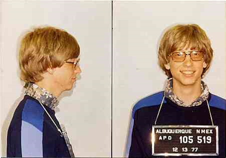
Nice guess!
 |
 |
|---|---|
| Biggest Ponzi scheme | Now a Billionaire |
Credit Scoring
- Mitigate the impact of credit risk and make more objective
and accurate decisions
- Estimate the risk of a customer defaulting his contracted
financial obligation if a loan is granted, based on past experiences
- Different machine learning methods are used in practice, and in the
literature: logistic regression, neural networks, discriminant analysis, genetic programing, decision trees, random forests among others
Credit Scoring
Formally, a credit score is a statistical model that allows the estimation of the probability of a customer $i$ defaulting a contracted debt ($y_i=1$)
$$\hat p_i=P(y_i=1|\mathbf{x}_i)$$
Example: Kaggle Credit Competition

Improve on the state of the art in credit scoring by predicting the probability that somebody will experience financial distress in the next two years.
Load dataset from CostCla package
from costcla.datasets import load_creditscoring1
data = load_creditscoring1()
Data file
print data.keys()
print 'Number of examples ', data.target.shape[0]
['target_names', 'cost_mat', 'name', 'DESCR', 'feature_names', 'data', 'target']
Number of examples  112915
Class Label
target = pd.DataFrame(pd.Series(data.target).value_counts(), columns=('Frequency',))
target['Percentage'] = target['Frequency'] / target['Frequency'].sum()
target.index = ['Negative (Good Customers)', 'Positive (Bad Customers)']
print target
                           Frequency  Percentage
Negative (Good Customers)     105299    0.932551
Positive (Bad Customers)        7616    0.067449
Features
pd.DataFrame(data.feature_names, columns=('Features',))
| Features | |
|---|---|
| 0 | RevolvingUtilizationOfUnsecuredLines |
| 1 | age |
| 2 | NumberOfTime30-59DaysPastDueNotWorse |
| 3 | DebtRatio |
| 4 | MonthlyIncome |
| 5 | NumberOfOpenCreditLinesAndLoans |
| 6 | NumberOfTimes90DaysLate |
| 7 | NumberRealEstateLoansOrLines |
| 8 | NumberOfTime60-89DaysPastDueNotWorse |
| 9 | NumberOfDependents |
Credit scoring as a classification problem
Split in training and testing
from sklearn.cross_validation import train_test_split
X_train, X_test, y_train, y_test, cost_mat_train, cost_mat_test = \
train_test_split(data.data, data.target, data.cost_mat)
Credit scoring as a classification problem
Fit models
from sklearn.ensemble import RandomForestClassifier
from sklearn.linear_model import LogisticRegression
from sklearn.tree import DecisionTreeClassifier

classifiers = {"RF": {"f": RandomForestClassifier()},
               "DT": {"f": DecisionTreeClassifier()},
               "LR": {"f": LogisticRegression()}}

# Fit the classifiers using the training dataset
for model in classifiers.keys():
    classifiers[model]["f"].fit(X_train, y_train)
    classifiers[model]["c"] = classifiers[model]["f"].predict(X_test)
    classifiers[model]["p"] = classifiers[model]["f"].predict_proba(X_test)
    classifiers[model]["p_train"] = classifiers[model]["f"].predict_proba(X_train)
Models performance
Evaluate metrics and plot results
from sklearn.metrics import f1_score, precision_score, recall_score, accuracy_score

measures = {"F1Score": f1_score, "Precision": precision_score,
            "Recall": recall_score, "Accuracy": accuracy_score}

results = pd.DataFrame(columns=measures.keys())

for model in classifiers.keys():
    results.loc[model] = [measures[measure](y_test, classifiers[model]["c"]) for measure in measures.keys()]
Models performance
fig1()

Models performance
- None of these measures takes into account the business and economical realities that take place in credit scoring.
- Costs that the financial institution had incurred to acquire customers, or the expected profit due to a particular client, are not considered in the evaluation of the different models.
Financial Evaluation of a Credit Scorecard
Motivation
- Typically, a credit risk model is evaluated using standard cost-insensitive measures.
- However, in practice, the cost associated with approving a bad customer (False Negative) is quite different from the cost associated with declining a good customer (False Positive).
- Furthermore, the costs are not constant among customers.
Cost Matrix
| | Actual Positive ($y_i=1$) | Actual Negative ($y_i=0$)| |--- |:-: |:-: | | Pred. Positive ($c_i=1$) | $C_{TP_i}=0$ | $C_{FP_i}=r_i+C^a_{FP}$ | | Pred. Negative ($c_i=0$) | $C_{FN_i}=Cl_i \cdot L_{gd}$ | $C_{TN_i}=0$ |
Where:
- $C_{FN_i}$ = losses if the customer $i$ defaults
- $Cl_i$ is the credi line of customer $i$
- $L_{gd}$ is the loss given default. Percentage of loss over the total credit line when the customer defaulted
Cost Matrix
- $C_{FP_i}=r_i+C^a_{FP}$
- $r_i$ is the loss in profit by rejecting what would have been a good customer.
- $C^a_{FP}$ is related to the assumption that the financial institution will not keep the money of the declined customer idle, but instead it will give
a loan to an alternative customer.
For more info see [Correa Bahnsen et al., 2014]
Parameters for the Kaggle Credit Database
Assuming the database belong to an average European financial institution, we find the different parameters needed to calculate the cost measure
| Parameter | Value | |--- |:-: | |Interest rate ($int_r$) | 4.79% | | Cost of funds ($int_{cf}$) | 2.94% | | Term ($l$) in months | 24 | | Loss given default ($L_{gd}$) | 75% | | Times income ($q$) | 3 | | Maximum credit line ($Cl_{max}$) | 25,000|
# The cost matrix is already calculated for the dataset
# cost_mat[C_FP,C_FN,C_TP,C_TN]
print data.cost_mat[[10, 17, 50]]
[[  1023.73054104  18750.              0.              0.        ]
 [   717.25781516   6749.25            0.              0.        ]
 [   866.65393177  12599.25            0.              0.        ]]
Financial savings
The financial cost of using a classifier $f$ on $\mathcal{S}$ is calculated by
$$ Cost(f(\mathcal{S})) = \sum_{i=1}^N y_i(1-c_i)C_{FN_i} + (1-y_i)c_i C_{FP_i}.$$
Then the financial savings are defined as the cost of the algorithm versus the cost of using no algorithm at all.
$$ Savings(f(\mathcal{S})) = \frac{ Cost_l(\mathcal{S}) - Cost(f(\mathcal{S}))} {Cost_l(\mathcal{S})},$$
where $Cost_l(\mathcal{S})$ is the cost of the costless class
Models Savings
costcla.metrics.savings_score(y_true, y_pred, cost_mat)
# Calculation of the cost and savings
from costcla.metrics import savings_score

# Evaluate the savings for each model
results["Savings"] = np.zeros(results.shape[0])
for model in classifiers.keys():
    results["Savings"].loc[model] = savings_score(y_test, classifiers[model]["c"], cost_mat_test)
Models Savings
fig2()

- There are significant differences in the results when evaluating a model using a traditional cost-insensitive measures
- ~17% of savings is very bad!
- Train models that take into account the different financial costs
Example-Dependent Cost-Sensitive Classification
*Why "Example-Dependent"
Cost-sensitive classification ussualy refers to class-dependent costs, where the cost dependends on the class but is assumed constant accross examples.
In credit scoring, different customers have different credit lines, which implies that the costs are not constant
Bayes Minimum Risk (BMR)
The BMR classifier is a decision model based on quantifying tradeoffs between various decisions using probabilities and the costs that accompany such decisions.
In particular:
$$ R(c_i=0|\mathbf{x}_i)=C_{TN_i}(1-\hat p_i)+C_{FN_i} \cdot \hat p_i, $$and $$ R(c_i=1|\mathbf{x}_i)=C_{TP_i} \cdot \hat p_i + C_{FP_i}(1- \hat p_i), $$
BMR Code
costcla.models.BayesMinimumRiskClassifier(calibration=True)
fit(y_true_cal=None, y_prob_cal=None)
- Parameters
- y_true_cal : True class
- y_prob_cal : Predicted probabilities
predict(y_prob,cost_mat)
Parameters
- y_prob : Predicted probabilities
- cost_mat : Cost matrix of the classification problem.
Returns
- y_pred : Predicted class
BMR Code
from costcla.models import BayesMinimumRiskClassifier
ci_models = classifiers.keys()

for model in ci_models:
    classifiers[model+"-BMR"] = {"f": BayesMinimumRiskClassifier()}
    # Fit
    classifiers[model+"-BMR"]["f"].fit(y_test, classifiers[model]["p"])
    # Calibration must be made in a validation set
    # Predict
    classifiers[model+"-BMR"]["c"] = classifiers[model+"-BMR"]["f"].predict(classifiers[model]["p"], cost_mat_test)
BMR Results
fig2()

BMR Results
- Bayes Minimum Risk increases the savings by using a cost-insensitive method and then introducing the costs
- Why not introduce the costs during the estimation of the methods?
Cost-Sensitive Decision Trees (CSDT)
A a new cost-based impurity measure taking into account the costs when all the examples in a leaf
costcla.models.CostSensitiveDecisionTreeClassifier(criterion='direct_cost', criterion_weight=False, pruned=True)
Cost-Sensitive Random Patches (CSRP)
Ensemble of CSDT
costcla.models.CostSensitiveRandomPatchesClassifier(n_estimators=10, max_samples=0.5, max_features=0.5,combination='majority_voting)
CSDT & CSRP Code
from costcla.models import CostSensitiveDecisionTreeClassifier
from costcla.models import CostSensitiveRandomPatchesClassifier

classifiers = {"CSDT": {"f": CostSensitiveDecisionTreeClassifier()},
               "CSRP": {"f": CostSensitiveRandomPatchesClassifier()}}

# Fit the classifiers using the training dataset
for model in classifiers.keys():
    classifiers[model]["f"].fit(X_train, y_train, cost_mat_train)
    classifiers[model]["c"] = classifiers[model]["f"].predict(X_test)
CSDT & CSRP Results
fig2()

Lessons Learned (so far ...)
- Selecting models based on traditional statistics does not give the best results in terms of cost
- Models should be evaluated taking into account real financial costs of the application
- Algorithms should be developed to incorporate those financial costs
CostCla Library
CostCla is a Python open source cost-sensitive classification library built on top of Scikit-learn, Pandas and Numpy.
Source code, binaries and documentation are distributed under 3-Clause BSD license in the website http://albahnsen.com/CostSensitiveClassification/
CostCla Algorithms
Cost-proportionate over-sampling [Elkan, 2001]
SMOTE [Chawla et al., 2002]
Cost-proportionate rejection-sampling [Zadrozny et al., 2003]
Thresholding optimization [Sheng and Ling, 2006]
Bayes minimum risk [Correa Bahnsen et al., 2014a]
Cost-sensitive logistic regression [Correa Bahnsen et al., 2014b]
Cost-sensitive decision trees [Correa Bahnsen et al., 2015a]
Cost-sensitive ensemble methods: cost-sensitive bagging, cost-sensitive pasting, cost-sensitive random forest and cost-sensitive random patches [Correa Bahnsen et al., 2015c]
CostCla Databases
Credit Scoring1 - Kaggle credit competition [Data], cost matrix: [Correa Bahnsen et al., 2014]
Credit Scoring 2 - PAKDD2009 Credit [Data], cost matrix: [Correa Bahnsen et al., 2014a]
Direct Marketing - PAKDD2009 Credit [Data], cost matrix: [Correa Bahnsen et al., 2014b]
Churn Modeling, June 2015
Future Work
- CSDT in Cython
- Cost-sensitive class-dependent algorithms
- Sampling algorithms
- Probability calibration (Only ROCCH)
- Compatibility with Python $\ge$ 3.4
- Other algorithms
- More databases
You find the presentation and the IPython Notebook here:
albahnsen/CostSensitiveClassification/blob/ master/doc/tutorials/slides_edcs_credit_scoring.ipynb#/
This slides are a short version of this tutorial: