10 - Perceptron Training
by Fabio A. González, Universidad Nacional de Colombia
version 1.0, June 2018
Part of the class Applied Deep Learning
This notebook is licensed under a Creative Commons Attribution-ShareAlike 3.0 Unported License.
Two Class Classification Problem
X, Y = make_blobs(n_samples=100, centers=2, n_features=2, random_state=0)
pl.figure(figsize=(8, 6))
plot_data(X, Y)

How to solve it?
- We need to design a prediction function $f:\mathbb{R}^{2}\rightarrow\mathbb{R}$ such that:
- Here we will model $f$ as a logistic model with parameters $w$ and $w_0$:
where $$\sigma(x) = \frac{1}{1+e^{-x}}$$
Perceptron
This model corresponds to a perceptron or logistic regression model
$$f_w(x,y) = P(C_1|x)= \sigma(wx+w_0)$$where $$\sigma(x) = \frac{1}{1+e^{-x}}$$
def sigmoid(x):
    return 1.0/(1.0 + np.exp(-x))

def predict(w, x):
    a = np.dot(w[1:], x) + w[0]
    z = sigmoid(a)
    return z
Learning as optimization
- General optimization problem:
- Hypothesis space:
- Cross entropy loss function:
- Measures the likelihood of the the probabilistic model represented by $f$ given the data $D$.
Calculating the cross entropy loss
def xentropy_loss(w, x, y):
    return - y * np.log(predict(w, x)) - (1 - y) * np.log(1 - predict(w, x))

def batch_loss(loss_fun, w, X, Y, ):
    n = X.shape[0]
    tot_loss = 0
    for i in range(n):
        tot_loss += loss_fun(w, X[i], Y[i])
    return tot_loss
plot_loss(bloss_xe)

Other loss fuctions
There are several different loss functions.
$L_1$ loss:
- $L_2$ loss:
pl.figure(figsize = (15,5))
pl.subplot(1,3,1); plot_loss(bloss_xe); pl.title("XE loss")
pl.subplot(1,3,2); pl.title("L1 loss"); plot_loss(loss1)
pl.subplot(1,3,3); pl.title("L2 loss"); plot_loss(loss2)

How to solve the learning problem?
- There are different optimization strategies:
- Linear optimization
- Convex optimization
- Non-linear optimization
- Combinatorial optimization
- No unique optimization strategy that works for all the problems: "no free lunch theorem"
How to solve the learning problem? (cont.)
- Trade-offs:
- Global optimum guarantee
- Simplicity of the method
- Easy parameter tuning
- Scalability
- Potential parallelization
- In machine learning preferences change over time.
- Nowadays scalable, easy parallelizable strategies are preferred even at the expense of guaranteed optimality.
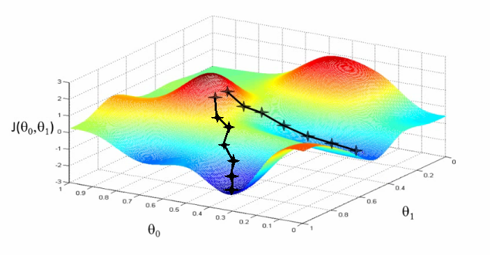
Gradient descent
Logistic regression gradient
$$ \begin{aligned}L(f,D) & = \sum_{(x_{i},r_{i})\in D} -r_i\log(f(x_i)) -(1-r_i)\log(1 - f(x_i))\\ & =\sum_{(x_{i},r_{i})\in D}E(w, x_i, r_i) \end{aligned} $$If $f_w$ is the sigmoid function: $$ \frac{\partial E(w,x_{i,}r_{i})}{\partial w}=(f_{w}(x_{i})-r_{i})x_{i} $$
def de_dw(w, x, r):
    x_prime = np.zeros(len(x) + 1)
    x_prime[1:] = x
    x_prime[0] = 1
    return (predict(w, x) - r) * x_prime
Checking the gradient calculation
"During the last twenty years, I have often been approached for advice in setting the learning rates γt of some rebellious stochastic gradient descent program. My advice is to forget about the learning rates and check that the gradients are computed correctly."
Bottou, L. (2012). Stochastic gradient descent tricks. In Neural networks: Tricks of the trade (pp. 421-436). Springer Berlin Heidelberg.
Checking the gradient calculation
def num_de_dw(w, x, y, epsilon):
    deltas = np.identity(len(w)) * epsilon
    de = np.zeros(len(w))
    for i in range(len(w)):
        de[i] = (xentropy_loss(w + deltas[i, :], x, y) - xentropy_loss(w - deltas[i, :], x, y)) / (2 * epsilon)
    return de

def test_de_dw():
    num_tests = 100
    epsilon = 0.0001
    for i in range(num_tests):
        tw = np.random.randn(3)
        tx = np.random.randn(2)
        ty = np.random.randn(1)
        if np.linalg.norm(de_dw(tw, tx,ty) - num_de_dw(tw, tx, ty, epsilon)) > epsilon:
            raise Exception("de_dw test failed!")
test_de_dw()
---------------------------------------------------------------------------
Exception                                 Traceback (most recent call last)
<ipython-input-77-af1997b0aa7e> in <module>()
----> 1 test_de_dw()

<ipython-input-50-489115583664> in test_de_dw()
     14         ty = np.random.randn(1)
     15         if np.linalg.norm(de_dw(tw, tx,ty) - num_de_dw(tw, tx, ty, epsilon)) > epsilon:
---> 16             raise Exception("de_dw test failed!")
     17

Exception: de_dw test failed!
Batch gradient descent
def batch_gd(X, Y, epochs, eta, w_ini):
    losses = []
    w = w_ini
    n = X.shape[0]
    for i in range(epochs):
        delta = np.zeros(len(w))
        for j in range(n):
            delta += de_dw(w, X[j], Y[j])
        w = w - eta * delta
        losses.append(batch_loss(xentropy_loss,w, X, Y))
    return w, losses
w, losses = batch_gd(X, Y, 50, 0.01, np.array([0, 0, 0]))
pl.figure(figsize = (8,16/3))
pl.plot(losses)
[<matplotlib.lines.Line2D at 0x11ba264e0>]

Online (stochastic) gradient descent
def sgd(X, Y, epochs, eta, w_ini):
    losses = []
    w = w_ini
    n = X.shape[0]
    for i in range(epochs):
        for j in range(n):
            delta = de_dw(w, X[j], Y[j])
            w = w - eta * delta
        losses.append(batch_loss(xentropy_loss,w, X, Y))
    return w, losses
lr = 0.005
epochs = 500
w1, losses_bt = batch_gd(X, Y, epochs, lr, np.array([0, 0, 0]))
w2, losses_ol = sgd(X, Y, epochs, lr, np.array([0, 0, 0]))
pl.figure(figsize = (8,16/3))
pl.plot(np.arange(epochs), losses_ol, label="SGD")
pl.plot(np.arange(epochs), losses_bt, label="Batch")
pl.xlabel("Epoch")
pl.ylabel("Loss")
pl.legend()
<matplotlib.legend.Legend at 0x11ccfbd30>

def gen_pred_fun(w):
    def pred_fun(x1, x2):
        x = np.array([x1, x2])
        return predict(w, x)
    return pred_fun

pl.figure(figsize = (8,16/3))
plot_decision_region(X, gen_pred_fun(w1))
plot_data(X, Y)
