#!/usr/bin/env python
# coding: utf-8
# # Application of MPBNs to the Th-differentiation model by Abou-Jaoudé et al. 2015
#
# We use Most Permissive Boolean Networks to reproduce the analyses the logical model published in
# [(Abou-Jaoudé et al., 2015)](https://doi.org/10.3389/fbioe.2014.00086)
# which focus on reprogramming capabilities accross different T-cell types.
# In[1]:
import biolqm
import ginsim
import pandas as pd
from functools import reduce
# In[2]:
import mpbn
# ## Model
#
# ### Original large-scale multivalued model
# In[3]:
lrg = ginsim.load("https://zenodo.org/record/3719059/files/Frontiers-Th-Full-model-annotated.zginml?download=1")
ginsim.show(lrg)
# We use `biolqm` to convert it to a pure Boolean model.
# In[4]:
bn = biolqm.to_minibn(biolqm.booleanize(lrg.getModel()))
inputs = set(bn.inputs())
len(bn), len(inputs)
# The following code cells define the different subtypes and conditions as specified in the article.
#
# ### Markers for T-cell subtypes
#
# The study list various T-cell subtypes which can be identified by particular combinations of markers activities. They are specified in the [Table 2 of article](https://doi.org/10.3389/fbioe.2014.00086), reproduced herebelow:
# 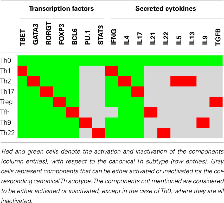 # In[5]:
subtypes = {
"Th0": (set(),set(bn)), # all nodes are inactive
"Th1": ({"TBET", "IFNG"},
{"GATA3", "RORGT", "FOXP3", "BCL6", "IL4", "IL17"}),
"Th2": ({"GATA3", "IL4", "IL5", "IL13"},
{"TBET", "RORGT", "FOXP3", "BCL6", "IFNG", "IL17"}),
"Th17": ({"RORGT", "IL17"},
{"TBET", "GATA3", "FOXP3", "BCL6", "IFNG", "IL4"}),
"Treg": ({"FOXP3", "TGFB"},
{"TBET", "GATA3", "RORGT", "BCL6", "IFNG", "IL4", "IL17"}),
"Tfh": ({"BCL6", "IL21"},
{"TBET", "GATA3", "RORGT", "FOXP3", "IL4", "IL17"}),
"Th9": ({"PU1", "IL9"},
{"TBET", "GATA3", "RORGT", "FOXP3", "BCL6", "IFNG", "IL4", "IL17"}),
"Th22": ({"STAT3", "IL22"},
{"TBET", "GATA3", "RORGT", "FOXP3", "BCL6", "IFNG", "IL4", "IL17"}),
}
#sanity check
for t, nodes in subtypes.items():
assert nodes[0].issubset(bn) and nodes[1].issubset(bn), \
"unknown nodes for {}".format(t)
# convert to configurations
def subtype_cfg(t):
return dict([(n, 1) for n in subtypes[t][0]] \
+ [(n, 0) for n in subtypes[t][1]])
subtypes = dict([(t, subtype_cfg(t)) for t in subtypes])
types = list(subtypes.keys())
# In[6]:
# display
tcolumns = ["TBET","GATA3","RORGT","FOXP3","BCL6","PU1","STAT3",
"IFNG","IL4","IL17","IL21","IL22","IL5","IL13","IL9","TGFB"]
assert len(tcolumns)==16,len(tcolumns)
def colordf(df):
def colorize(val):
if val == 1:
return "color: red; background-color: red"
if val == 0:
return "color: lime; background-color: lime"
if val == "*":
return "color: lightgrey; background-color: lightgrey"
return ""
return df.style.applymap(colorize)
types = list(subtypes.keys())
df = pd.DataFrame([subtypes[t] for t in types], index=types, columns=tcolumns).fillna('*')
colordf(df)
# ### Input conditions
#
# The study relies on a set of input conditions for the network which should trigger cell type transdifferentiation. They are specified in the [Table 3 of article](https://doi.org/10.3389/fbioe.2014.00086), reproduced herebelow:
#
# In[5]:
subtypes = {
"Th0": (set(),set(bn)), # all nodes are inactive
"Th1": ({"TBET", "IFNG"},
{"GATA3", "RORGT", "FOXP3", "BCL6", "IL4", "IL17"}),
"Th2": ({"GATA3", "IL4", "IL5", "IL13"},
{"TBET", "RORGT", "FOXP3", "BCL6", "IFNG", "IL17"}),
"Th17": ({"RORGT", "IL17"},
{"TBET", "GATA3", "FOXP3", "BCL6", "IFNG", "IL4"}),
"Treg": ({"FOXP3", "TGFB"},
{"TBET", "GATA3", "RORGT", "BCL6", "IFNG", "IL4", "IL17"}),
"Tfh": ({"BCL6", "IL21"},
{"TBET", "GATA3", "RORGT", "FOXP3", "IL4", "IL17"}),
"Th9": ({"PU1", "IL9"},
{"TBET", "GATA3", "RORGT", "FOXP3", "BCL6", "IFNG", "IL4", "IL17"}),
"Th22": ({"STAT3", "IL22"},
{"TBET", "GATA3", "RORGT", "FOXP3", "BCL6", "IFNG", "IL4", "IL17"}),
}
#sanity check
for t, nodes in subtypes.items():
assert nodes[0].issubset(bn) and nodes[1].issubset(bn), \
"unknown nodes for {}".format(t)
# convert to configurations
def subtype_cfg(t):
return dict([(n, 1) for n in subtypes[t][0]] \
+ [(n, 0) for n in subtypes[t][1]])
subtypes = dict([(t, subtype_cfg(t)) for t in subtypes])
types = list(subtypes.keys())
# In[6]:
# display
tcolumns = ["TBET","GATA3","RORGT","FOXP3","BCL6","PU1","STAT3",
"IFNG","IL4","IL17","IL21","IL22","IL5","IL13","IL9","TGFB"]
assert len(tcolumns)==16,len(tcolumns)
def colordf(df):
def colorize(val):
if val == 1:
return "color: red; background-color: red"
if val == 0:
return "color: lime; background-color: lime"
if val == "*":
return "color: lightgrey; background-color: lightgrey"
return ""
return df.style.applymap(colorize)
types = list(subtypes.keys())
df = pd.DataFrame([subtypes[t] for t in types], index=types, columns=tcolumns).fillna('*')
colordf(df)
# ### Input conditions
#
# The study relies on a set of input conditions for the network which should trigger cell type transdifferentiation. They are specified in the [Table 3 of article](https://doi.org/10.3389/fbioe.2014.00086), reproduced herebelow:
# 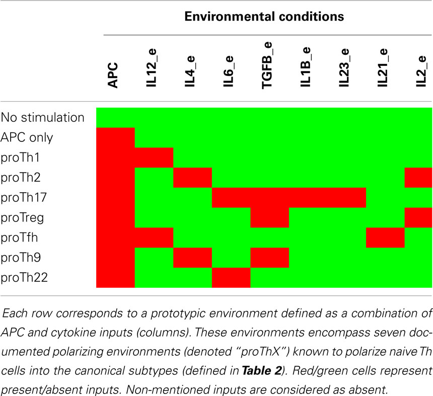 #
# **Warning** The `proTh9` condition requires an active `IL15_e`, which is not mentioned in the paper. Without it, there is no stable state matching with the condition, which seems a mistake.
# In[7]:
conditions = {
"idle": set(),
"APC": {"APC"},
"proTh1": {"APC", "IL12_e"},
"proTh2": {"APC", "IL4_e", "IL2_e"},
"proTh17": {"APC", "IL6_e", "TGFB_e", "IL1B_e", "IL23_e"},
"proTreg": {"APC", "TGFB_e", "IL2_e"},
"proTfh": {"APC", "IL12_e", "IL21_e"},
"proTh9": {"APC", "IL4_e", "TGFB_e", "IL15_e"}, # warning IL15_e is necessary!
"proTh22": {"APC", "IL6_e"},
}
condition_nodes = reduce(set.union, conditions.values())
# sanity check
for nodes in conditions.values():
assert set(nodes).issubset(inputs), \
"unknown nodes in {}".format(nodes)
def condition_cfg(t):
return dict([(n, 1) for n in conditions[t]] \
+ [(n, 0) for n in (inputs - set(conditions[t]))])
conditions = dict([(c, condition_cfg(c)) for c in conditions])
# In[8]:
# display
ecolumns = ["APC","IL12_e","IL4_e","IL6_e","TGFB_e","IL1B_e","IL23_e","IL21_e","IL2_e","IL15_e"]
key_conditions = list(conditions.keys())
df = pd.DataFrame([conditions[c] for c in key_conditions], index=key_conditions, columns=ecolumns)
colordf(df)
# ### Reprogramming graph
#
# The core of the study lies on the prediction of reprogramming conditions accross the different subtypes. It results in a graph given in the [Figure 3 of article](https://doi.org/10.3389/fbioe.2014.00086), reproduced herebelow:
#
#
#
# **Warning** The `proTh9` condition requires an active `IL15_e`, which is not mentioned in the paper. Without it, there is no stable state matching with the condition, which seems a mistake.
# In[7]:
conditions = {
"idle": set(),
"APC": {"APC"},
"proTh1": {"APC", "IL12_e"},
"proTh2": {"APC", "IL4_e", "IL2_e"},
"proTh17": {"APC", "IL6_e", "TGFB_e", "IL1B_e", "IL23_e"},
"proTreg": {"APC", "TGFB_e", "IL2_e"},
"proTfh": {"APC", "IL12_e", "IL21_e"},
"proTh9": {"APC", "IL4_e", "TGFB_e", "IL15_e"}, # warning IL15_e is necessary!
"proTh22": {"APC", "IL6_e"},
}
condition_nodes = reduce(set.union, conditions.values())
# sanity check
for nodes in conditions.values():
assert set(nodes).issubset(inputs), \
"unknown nodes in {}".format(nodes)
def condition_cfg(t):
return dict([(n, 1) for n in conditions[t]] \
+ [(n, 0) for n in (inputs - set(conditions[t]))])
conditions = dict([(c, condition_cfg(c)) for c in conditions])
# In[8]:
# display
ecolumns = ["APC","IL12_e","IL4_e","IL6_e","TGFB_e","IL1B_e","IL23_e","IL21_e","IL2_e","IL15_e"]
key_conditions = list(conditions.keys())
df = pd.DataFrame([conditions[c] for c in key_conditions], index=key_conditions, columns=ecolumns)
colordf(df)
# ### Reprogramming graph
#
# The core of the study lies on the prediction of reprogramming conditions accross the different subtypes. It results in a graph given in the [Figure 3 of article](https://doi.org/10.3389/fbioe.2014.00086), reproduced herebelow:
#
# 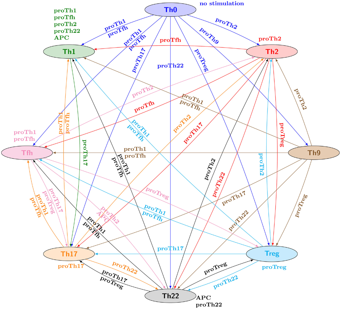 #
# There is an edge from type T1 to T2 labeled with an input condition E whenever from any configuration matching with T1 markers there exists a path to an attractor matching with T2 under the steady input condition E.
#
# The cell below lists the reprogramming paths of the above graph.
# In[9]:
orig_reprogramming = {'Th0': {
'Th1': {'proTfh', 'proTh1'},
'Tfh': {'proTfh', 'proTh1'},
'Th9': {'proTh9'},
'Th2': {'proTh2'},
'Th17': {'proTh17'},
'Treg': {'proTreg'},
'Th22': {'proTh22'}},
'Th1': {
'Th1': {'APC', 'proTfh', 'proTh1', 'proTh2', 'proTh22'},
'Th17': {'proTh17'}},
'Th2': {
'Th2': {'proTh2'},
'Th1': {'proTfh'},
'Tfh': {'proTfh'},
'Th17': {'proTh17'},
'Treg': {'proTreg'},
'Th22': {'proTh22'}},
'Tfh': {
'Tfh': {'proTfh', 'proTh1'},
'Th22': {'APC', 'proTh22'},
'Th2': {'proTh2'},
'Th17': {'proTh17', 'proTreg'},
'Treg': {'proTreg'}},
'Th17': {
'Th17': {'proTh17'},
'Th22': {'proTh22'},
'Th1': {'proTfh', 'proTh1'},
'Tfh': {'proTfh', 'proTh1'},
'Th2': {'proTh2'}},
'Treg': {
'Treg': {'proTreg'},
'Th1': {'proTfh', 'proTh1'},
'Tfh': {'proTfh', 'proTh1'},
'Th2': {'proTh2'},
'Th17': {'proTh17'},
'Th22': {'proTh22'}},
'Th9': {
'Th2': {'proTh2'},
'Th1': {'proTfh', 'proTh1'},
'Tfh': {'proTfh', 'proTh1'},
'Th17': {'proTh17'},
'Th22': {'proTh22'},
'Treg': {'proTreg'}},
'Th22': {
'Th22': {'APC', 'proTh22'},
'Th1': {'proTfh', 'proTh1'},
'Tfh': {'proTfh', 'proTh1'},
'Th2': {'proTh2'},
'Th17': {'proTh17', 'proTreg'},
'Treg': {'proTreg'}}}
# ## Analysis with MPBNs
# ### Model import and helper functions
# We convert the Boolean model to MPBN.
# In[10]:
mbn = mpbn.MPBooleanNetwork(bn)
# Herebelow are helper functions for the analysis.
# In[11]:
def apply_condition(cfg, c):
ccfg = cfg.copy()
for n, v in conditions[c].items():
ccfg[n] = v
for n in [n for n, v in ccfg.items() if v == '*']:
del ccfg[n]
return ccfg
def trigger_subtype(t, c):
return apply_condition(subtypes[t], c)
def match_subtype(cfg, t):
markers = subtypes[t]
cyclic = []#[n for (n,v) in cfg.items() if v == '*']
if cyclic:
cfg = cfg.copy()
for n in cyclic:
cfg[n] = markers.get(n)
return set(markers.items()).issubset(set(cfg.items()))
def label_subtype(cfg):
for t in subtypes:
if match_subtype(cfg, t):
return t
def labels(a_it):
ls = set([label_subtype(a) for a in a_it])
ls.discard(None)
return ls
# ### Computation of attractors
#
# Let us first compute the list of attractors under each defined conditions:
# In[12]:
get_ipython().run_line_magic('time', 'attractors = dict([(c, list(mbn.attractors(constraints=conditions[c]))) for c in conditions])')
# To analyse the nature of attractors, we filter the fixed point from the above list.
# In[13]:
fixpoints = dict([(c, [x for x in ts if "*" not in x.values()]) \
for (c,ts) in attractors.items()])
# For each condition, we display the count of attractors, and the count of fixed points.
# In[14]:
dict([(c, (len(attractors[c]),len(fixpoints[c]))) for c in conditions])
# Thus, it results that all the attractors of the devised input conditions are actually fixed points. MPBNs allow to conclude that there is *no cyclic attractor*, even with asynchronous interpretation.
#
# We now classify the attractors by subtype, and display their count.
# In[15]:
attractors_by_subtype=dict([(t,[]) for t in subtypes])
for ts in attractors.values():
for x in ts:
t = label_subtype(x)
if t is None:
continue
attractors_by_subtype[t].append(x)
attractors_by_subtype["Th0"].append(subtypes["Th0"])
dict([(t,len(ts)) for (t,ts) in attractors_by_subtype.items()])
# ### Computation of the reprogramming graph
#
# We divide the assessment of reprogramming paths from subtypes T1 to T2 under input conditions E in two steps:
# 1. we first consider initial configurations which are in an attractor of T1, and check whever applying E enable the reachability of an attractor of T2;
# 2. if true, we look for counter examples where there exists an initial configuration matching T1 but not necessarily in an attractor which cannot reach an attractor of T2.
#
# #### Step 1
#
# The algorithm of step 1 is the following:
# - for each subtype t
# - for each input condition c
# 1. for each attractor x of subtype t
# 1. compute the reachable attractors from a configuration matching with x with condition c
# 2. assign the subtype for each reached attractor (ls[x])
# 2. there is an edge from t to l with label c whenever the type l has been always reached
#
# Notice the computation time.
# In[16]:
get_ipython().run_cell_magic('time', '', 'rg = {}\nfor t in subtypes:\n rg[t] = {}\n for c in conditions:\n if c == "idle":\n continue\n ls = [labels(mbn.attractors(reachable_from=apply_condition(x,c))) \\\n for x in attractors_by_subtype[t]]\n if not ls:\n continue\n ls = reduce(set.intersection, ls)\n for l in ls:\n if l not in rg[t]:\n rg[t][l] = set()\n rg[t][l].add(c)\n')
# #### Step 2
#
# The authors of the original study consider *any* initial configuration matching a subtype T1, not necessarily those belonging to an attractor of T1.
# Therefore, the graph computed above can be over-estimated: there may exists non-stable configurations matching with T1 where applying the condition E does not lead to the subtype T2.
#
# To find such counter-examples, we rely on a preview of an in-development tool which provides more features than the simple `mpbn` library.
# In[17]:
# manual installation of bonesis preview code
get_ipython().system('curl -o /tmp/bonesis.zip https://zenodo.org/record/3715210/files/bonesis-preview-20200318.zip?download=1')
get_ipython().system('mkdir -p /tmp/bonesis')
from zipfile import ZipFile
with ZipFile("/tmp/bonesis.zip") as z:
z.extractall("/tmp/bonesis/")
import sys
sys.path.insert(0, "/tmp/bonesis")
# In[18]:
import bonesis0
from bonesis0.proxy_control import ProxyControl
from bonesis0.utils import aspf
import clingo
# In[19]:
def has_nonreach(t1, e, t2):
"""
Returns True whenever there exists a configuration matching with t1
for which none of the attractor of t2 are reachable when applying conditin e
"""
def make_obs(name, cfg):
fs = [f"obs({name},\"{node}\",{2*v-1})." for node, v in cfg.items() if v != '*']
return "\n".join(fs)
control = ProxyControl(["-c", "bounded_nonreach=1", "1"])
control.add("base", [], mbn.asp_of_bn())
control.load(aspf("eval.asp"))
control.load(aspf("complete-cfg.asp"))
control.load(aspf("reach.asp"))
control.load(aspf("nonreach.asp"))
control.add("base", [], make_obs("init", apply_condition(subtypes[t1], e)))
for i, cfg in enumerate(attractors_by_subtype[t2]):
control.add("base", [], make_obs(f"dest{i}", cfg))
control.add("base", [], f"nonreach(init, dest{i}).")
control.ground([("base",[])])
return control.solve().satisfiable
# In[20]:
get_ipython().run_cell_magic('time', '', 'for c1 in rg:\n ftodel = []\n for c2, es in rg[c1].items():\n todel = []\n for e in es:\n if has_nonreach(c1, e, c2):\n todel.append(e)\n print(f"counter-example found for {c1} -({e})-> {c2}")\n for e in todel:\n es.remove(e)\n if not es:\n ftodel.append(c2)\n for c2 in ftodel:\n del rg[c1][c2]\n')
# ### Summary
#
# Let us now compare the obtained graph with the graph from the original study:
# In[21]:
rg == orig_reprogramming
# In[ ]:
#
# There is an edge from type T1 to T2 labeled with an input condition E whenever from any configuration matching with T1 markers there exists a path to an attractor matching with T2 under the steady input condition E.
#
# The cell below lists the reprogramming paths of the above graph.
# In[9]:
orig_reprogramming = {'Th0': {
'Th1': {'proTfh', 'proTh1'},
'Tfh': {'proTfh', 'proTh1'},
'Th9': {'proTh9'},
'Th2': {'proTh2'},
'Th17': {'proTh17'},
'Treg': {'proTreg'},
'Th22': {'proTh22'}},
'Th1': {
'Th1': {'APC', 'proTfh', 'proTh1', 'proTh2', 'proTh22'},
'Th17': {'proTh17'}},
'Th2': {
'Th2': {'proTh2'},
'Th1': {'proTfh'},
'Tfh': {'proTfh'},
'Th17': {'proTh17'},
'Treg': {'proTreg'},
'Th22': {'proTh22'}},
'Tfh': {
'Tfh': {'proTfh', 'proTh1'},
'Th22': {'APC', 'proTh22'},
'Th2': {'proTh2'},
'Th17': {'proTh17', 'proTreg'},
'Treg': {'proTreg'}},
'Th17': {
'Th17': {'proTh17'},
'Th22': {'proTh22'},
'Th1': {'proTfh', 'proTh1'},
'Tfh': {'proTfh', 'proTh1'},
'Th2': {'proTh2'}},
'Treg': {
'Treg': {'proTreg'},
'Th1': {'proTfh', 'proTh1'},
'Tfh': {'proTfh', 'proTh1'},
'Th2': {'proTh2'},
'Th17': {'proTh17'},
'Th22': {'proTh22'}},
'Th9': {
'Th2': {'proTh2'},
'Th1': {'proTfh', 'proTh1'},
'Tfh': {'proTfh', 'proTh1'},
'Th17': {'proTh17'},
'Th22': {'proTh22'},
'Treg': {'proTreg'}},
'Th22': {
'Th22': {'APC', 'proTh22'},
'Th1': {'proTfh', 'proTh1'},
'Tfh': {'proTfh', 'proTh1'},
'Th2': {'proTh2'},
'Th17': {'proTh17', 'proTreg'},
'Treg': {'proTreg'}}}
# ## Analysis with MPBNs
# ### Model import and helper functions
# We convert the Boolean model to MPBN.
# In[10]:
mbn = mpbn.MPBooleanNetwork(bn)
# Herebelow are helper functions for the analysis.
# In[11]:
def apply_condition(cfg, c):
ccfg = cfg.copy()
for n, v in conditions[c].items():
ccfg[n] = v
for n in [n for n, v in ccfg.items() if v == '*']:
del ccfg[n]
return ccfg
def trigger_subtype(t, c):
return apply_condition(subtypes[t], c)
def match_subtype(cfg, t):
markers = subtypes[t]
cyclic = []#[n for (n,v) in cfg.items() if v == '*']
if cyclic:
cfg = cfg.copy()
for n in cyclic:
cfg[n] = markers.get(n)
return set(markers.items()).issubset(set(cfg.items()))
def label_subtype(cfg):
for t in subtypes:
if match_subtype(cfg, t):
return t
def labels(a_it):
ls = set([label_subtype(a) for a in a_it])
ls.discard(None)
return ls
# ### Computation of attractors
#
# Let us first compute the list of attractors under each defined conditions:
# In[12]:
get_ipython().run_line_magic('time', 'attractors = dict([(c, list(mbn.attractors(constraints=conditions[c]))) for c in conditions])')
# To analyse the nature of attractors, we filter the fixed point from the above list.
# In[13]:
fixpoints = dict([(c, [x for x in ts if "*" not in x.values()]) \
for (c,ts) in attractors.items()])
# For each condition, we display the count of attractors, and the count of fixed points.
# In[14]:
dict([(c, (len(attractors[c]),len(fixpoints[c]))) for c in conditions])
# Thus, it results that all the attractors of the devised input conditions are actually fixed points. MPBNs allow to conclude that there is *no cyclic attractor*, even with asynchronous interpretation.
#
# We now classify the attractors by subtype, and display their count.
# In[15]:
attractors_by_subtype=dict([(t,[]) for t in subtypes])
for ts in attractors.values():
for x in ts:
t = label_subtype(x)
if t is None:
continue
attractors_by_subtype[t].append(x)
attractors_by_subtype["Th0"].append(subtypes["Th0"])
dict([(t,len(ts)) for (t,ts) in attractors_by_subtype.items()])
# ### Computation of the reprogramming graph
#
# We divide the assessment of reprogramming paths from subtypes T1 to T2 under input conditions E in two steps:
# 1. we first consider initial configurations which are in an attractor of T1, and check whever applying E enable the reachability of an attractor of T2;
# 2. if true, we look for counter examples where there exists an initial configuration matching T1 but not necessarily in an attractor which cannot reach an attractor of T2.
#
# #### Step 1
#
# The algorithm of step 1 is the following:
# - for each subtype t
# - for each input condition c
# 1. for each attractor x of subtype t
# 1. compute the reachable attractors from a configuration matching with x with condition c
# 2. assign the subtype for each reached attractor (ls[x])
# 2. there is an edge from t to l with label c whenever the type l has been always reached
#
# Notice the computation time.
# In[16]:
get_ipython().run_cell_magic('time', '', 'rg = {}\nfor t in subtypes:\n rg[t] = {}\n for c in conditions:\n if c == "idle":\n continue\n ls = [labels(mbn.attractors(reachable_from=apply_condition(x,c))) \\\n for x in attractors_by_subtype[t]]\n if not ls:\n continue\n ls = reduce(set.intersection, ls)\n for l in ls:\n if l not in rg[t]:\n rg[t][l] = set()\n rg[t][l].add(c)\n')
# #### Step 2
#
# The authors of the original study consider *any* initial configuration matching a subtype T1, not necessarily those belonging to an attractor of T1.
# Therefore, the graph computed above can be over-estimated: there may exists non-stable configurations matching with T1 where applying the condition E does not lead to the subtype T2.
#
# To find such counter-examples, we rely on a preview of an in-development tool which provides more features than the simple `mpbn` library.
# In[17]:
# manual installation of bonesis preview code
get_ipython().system('curl -o /tmp/bonesis.zip https://zenodo.org/record/3715210/files/bonesis-preview-20200318.zip?download=1')
get_ipython().system('mkdir -p /tmp/bonesis')
from zipfile import ZipFile
with ZipFile("/tmp/bonesis.zip") as z:
z.extractall("/tmp/bonesis/")
import sys
sys.path.insert(0, "/tmp/bonesis")
# In[18]:
import bonesis0
from bonesis0.proxy_control import ProxyControl
from bonesis0.utils import aspf
import clingo
# In[19]:
def has_nonreach(t1, e, t2):
"""
Returns True whenever there exists a configuration matching with t1
for which none of the attractor of t2 are reachable when applying conditin e
"""
def make_obs(name, cfg):
fs = [f"obs({name},\"{node}\",{2*v-1})." for node, v in cfg.items() if v != '*']
return "\n".join(fs)
control = ProxyControl(["-c", "bounded_nonreach=1", "1"])
control.add("base", [], mbn.asp_of_bn())
control.load(aspf("eval.asp"))
control.load(aspf("complete-cfg.asp"))
control.load(aspf("reach.asp"))
control.load(aspf("nonreach.asp"))
control.add("base", [], make_obs("init", apply_condition(subtypes[t1], e)))
for i, cfg in enumerate(attractors_by_subtype[t2]):
control.add("base", [], make_obs(f"dest{i}", cfg))
control.add("base", [], f"nonreach(init, dest{i}).")
control.ground([("base",[])])
return control.solve().satisfiable
# In[20]:
get_ipython().run_cell_magic('time', '', 'for c1 in rg:\n ftodel = []\n for c2, es in rg[c1].items():\n todel = []\n for e in es:\n if has_nonreach(c1, e, c2):\n todel.append(e)\n print(f"counter-example found for {c1} -({e})-> {c2}")\n for e in todel:\n es.remove(e)\n if not es:\n ftodel.append(c2)\n for c2 in ftodel:\n del rg[c1][c2]\n')
# ### Summary
#
# Let us now compare the obtained graph with the graph from the original study:
# In[21]:
rg == orig_reprogramming
# In[ ]: