#!/usr/bin/env python
# coding: utf-8

# # ENV/ATM 415: Climate Laboratory
# 
# [Brian E. J. Rose](http://www.atmos.albany.edu/facstaff/brose/index.html), University at Albany
# 
# # Lecture 16: The one-dimensional Energy Balance Model

# ## Contents
# 
# 1. [Heat transport and the energy budget for each latitude band](#section1)
# 2. [Parameterizing the radiation terms](#section2)
# 3. [Tuning the longwave parameters with reanalysis data](#section3)
# 4. [The one-dimensional diffusive energy balance model](#section4)
# 5. [The annual-mean EBM](#section5)
# 6. [Tuning the diffusivity](#section6)
# 7. [Summary: parameter values in the diffusive EBM](#section7)

# ____________
# <a id='section1'></a>
# 
# ## 1. Heat transport and the energy budget for each latitude band
# ____________

# Way back at the beginning of the semester we wrote down a **global average energy budget** that looked like
# 
# $$ C \frac{dT}{dt} = \text{ASR} - \text{OLR} $$

# Last time we talked about the additional **local heating** of each latitude band associated with atmospheric and oceanic motions:
# 
# $$ h = - \frac{1}{2 \pi a^2  \cos⁡\phi } \frac{\partial \mathcal{H}}{\partial \phi} $$

# Using this, we can write down a **local energy budget** expressing how the temperature of each latitude band should change:
# 
# $$ C \frac{\partial T}{\partial t} = \text{ASR} - \text{OLR} - \frac{1}{2 \pi a^2  \cos⁡\phi } \frac{\partial \mathcal{H}}{\partial \phi}$$

# Now the temperature $T$ is a function of latitude $\phi$ as well as time $t$ (so we write it as a partial derivative) 

# We also introduced the **diffusive heat transport parameterization**
# 
# $$ \mathcal{H}(\phi) = -2 \pi ~a^2 \cos\phi D \frac{\partial T}{\partial \phi} $$

# Putting this parameterization into the budget above gives
# 
# $$ C \frac{\partial T}{\partial t} = \text{ASR} - \text{OLR} + \frac{D}{\cos⁡\phi } \frac{\partial}{\partial \phi} \left( \cos\phi \frac{\partial T}{\partial \phi} \right)$$
# 
# (where we pulled the parameter $D$ out of the derivative because we are assuming it is a constant)

# ____________
# <a id='section2'></a>
# 
# ## 2. Parameterizing the radiation terms
# ____________

# To turn our **budget** into a **model**, we need specific parameterizations that link the radiation ASR and OLR to surface temperature $T$ (the state variable for our model).

# ### Fixed albedo assumption

# First, as usual, we can write the solar term as
# 
# $$ \text{ASR} = (1-\alpha) ~ Q $$

# For now, we will **assume that the planetary albedo is fixed (does not depend on temperature)**. Therefore the entire shortwave term $(1-\alpha) Q$ is a fixed source term in our budget. It varies in space and time but does not depend on $T$.

# Note that the solar term is (at least in annual average) larger at equator than poles… and transport term acts to flatten out the temperatures.

# ### Parameterizing the longwave radiation

# Now, we almost have a model we can solve for $T$!  Just need a function OLR$(T)$ expressing the temperature dependence of the emission to space.
# 
# So…  what’s the link between OLR and temperature????
# 
# [ discuss ]

# We spent a good chunk of the course looking at this question, and developed a model of a vertical column of air.
# 
# We are trying now to build a model of the equator-to-pole (or pole-to-pole) temperature structure.

# We COULD use an array of column models, representing temperature as a function of height and latitude (and time).
# 
# But instead, we will keep things simple, one spatial dimension at a time.

# Introduce the following **simple parameterization**:
# 
# $$ \text{OLR} = A + B T $$
# 
# With:
# 
# - $T$ the zonal average surface temperature in ºC
# - $A$ is a constant in W m$^{-2}$
# - $B$ is a constant in W m$^{-2}$ ºC$^{-1}$.
# 
# Think of $A$ as an inverse measure of the greenhouse gas amount (Why?).
# 
# The parameter $B$ is closely related to the **climate feedback parameter** $\lambda$ that we defined a while back. The only difference is that in the EBM we are going to explicitly separate the **albedo feedback** from all other radiative feedbacks.

# ____________
# <a id='section3'></a>
# 
# ## 3. Tuning the longwave parameters with reanalysis data
# ____________

# ### OLR versus surface temperature in NCEP Reanalysis data
# 
# Let's look at the data to find reasonable values for $A$ and $B$.

# In[1]:


get_ipython().run_line_magic('matplotlib', 'inline')
import numpy as np
import matplotlib.pyplot as plt
import xarray as xr
import climlab


# In[2]:


ncep_url = "http://www.esrl.noaa.gov/psd/thredds/dodsC/Datasets/ncep.reanalysis.derived/"
ncep_air = xr.open_dataset( ncep_url + "pressure/air.mon.1981-2010.ltm.nc", decode_times=False)
ncep_Ts = xr.open_dataset( ncep_url + "surface_gauss/skt.sfc.mon.1981-2010.ltm.nc", decode_times=False)
lat_ncep = ncep_Ts.lat; lon_ncep = ncep_Ts.lon
print( ncep_Ts)


# In[3]:


Ts_ncep_annual = ncep_Ts.skt.mean(dim=('lon','time'))


# In[4]:


ncep_ulwrf = xr.open_dataset( ncep_url + "other_gauss/ulwrf.ntat.mon.1981-2010.ltm.nc", decode_times=False)
ncep_dswrf = xr.open_dataset( ncep_url + "other_gauss/dswrf.ntat.mon.1981-2010.ltm.nc", decode_times=False)
ncep_uswrf = xr.open_dataset( ncep_url + "other_gauss/uswrf.ntat.mon.1981-2010.ltm.nc", decode_times=False)
OLR_ncep_annual = ncep_ulwrf.ulwrf.mean(dim=('lon','time'))
ASR_ncep_annual = (ncep_dswrf.dswrf - ncep_uswrf.uswrf).mean(dim=('lon','time'))


# In[5]:


from scipy.stats import linregress
slope, intercept, r_value, p_value, std_err = linregress(Ts_ncep_annual, OLR_ncep_annual)

print( 'Best fit is A = %0.0f W/m2 and B = %0.1f W/m2/degC' %(intercept, slope))


# We're going to plot the data and the best fit line, but also another line using these values:

# In[6]:


#  More standard values
A = 210.
B = 2.


# In[7]:


fig, ax1 = plt.subplots(figsize=(8,6))
ax1.plot( Ts_ncep_annual, OLR_ncep_annual, 'o' , label='data')
ax1.plot( Ts_ncep_annual, intercept + slope * Ts_ncep_annual, 'k--', label='best fit')
ax1.plot( Ts_ncep_annual, A + B * Ts_ncep_annual, 'r--', label='B=2')
ax1.set_xlabel('Surface temperature (C)', fontsize=16)
ax1.set_ylabel('OLR (W m$^{-2}$)', fontsize=16)
ax1.set_title('OLR versus surface temperature from NCEP reanalysis', fontsize=18)
ax1.legend(loc='upper left')
ax1.grid()


# Discuss these curves...
# 
# Suggestion of at least 3 different regimes with different slopes (cold, medium, warm).
# 
# Unbiased "best fit" is actually a poor fit over all the intermediate temperatures.
# 
# The astute reader will note that...   by taking the zonal average of the data before the regression, we are biasing this estimate toward cold temperatures.  [WHY?]
# 
# 

# Let's take these reference values:
# 
# $$ A = 210 ~ \text{W m}^{-2}, ~~~ B = 2 ~ \text{W m}^{-2}~^\circ\text{C}^{-1} $$

# Note that in the **global average**, recall $\overline{T_s} = 288 \text{ K} = 15^\circ\text{C}$
# 
# And so this parameterization gives 
# 
# $$ \overline{\text{OLR}} = 210 + 15 \times 2 = 240 ~\text{W m}^{-2} $$
# 
# And the observed global mean is $\overline{\text{OLR}} = 239 ~\text{W m}^{-2} $
# So this is consistent.
# 
# 
# 

# ### Relationship between $B$ and feedback parameters

# Recall that when we looked at climate forcing and feedback, we said that overall response to a forcing $\Delta R$ in W m$^{-2}$ is
# 
# $$ \Delta T = \frac{\Delta R}{\lambda} $$
# 
# and where $\lambda$ is the overall **climate feedback parameter**:
# 
# $$\lambda = \lambda_0 - \sum_{i=1}^{N} \lambda_i $$
# 
# and
# 
# - $\lambda_0 = 3.3$ W m$^{-2}$ K$^{-1}$ is the no-feedback climate response
# - $\sum_{i=1}^{N} \lambda_i$ is the sum of all radiative feedbacks, defined to be **positive** for **amplifying processes**.

# More positive feedbacks thus mean that $\lambda$ is a smaller number, which means the response to a given forcing is larger!

# Here in the EBM the parameter $B$ plays the same role as $\lambda$ -- a smaller number means a more sensitive model.

# Our estimate $B = 2 ~ \text{W m}^{-2}~^\circ\text{C}^{-1}$ thus implies that the sum of all LW feedback processes (including water vapor, lapse rates and clouds) is
# 
# $$ \sum_{i=1}^{N} \lambda_i = 3.3 ~\text{W m}^{-2}~^\circ\text{C}^{-1} - 2 ~\text{W m}^{-2}~^\circ\text{C}^{-1} = 1.3 ~\text{W m}^{-2}~^\circ\text{C}^{-1} $$ 

# Looking back at the chart of feedback parameter values from GCMs, does this seem plausible?

# ____________
# <a id='section4'></a>
# 
# ## 4. The one-dimensional diffusive energy balance model
# ____________
# 
# 

# Putting the above OLR parameterization into our budget equation gives
# 
# $$ C \frac{\partial T}{\partial t} = (1-\alpha) ~ Q - \left( A + B~T \right) + \frac{D}{\cos⁡\phi } \frac{\partial }{\partial \phi} \left(   \cos⁡\phi  ~ \frac{\partial T}{\partial \phi} \right) $$

# This is the equation for a very important and useful simple model of the climate system. It is typically referred to as the (one-dimensional) Energy Balance Model.
# 
# (although as we have seen over and over, EVERY climate model is actually an “energy balance model” of some kind)
# 
# Also for historical reasons this is often called the **Budyko-Sellers model**, after Budyko and Sellers who both (independently of each other) published influential papers on this subject in 1969.

# Recap: parameters in this model are
# 
# - C: heat capacity in J m$^{-2}$ ºC$^{-1}$
# - A: longwave emission at 0ºC in W m$^{-2}$
# - B: increase in emission per degree, in W m$^{-2}$ ºC$^{-1}$
# - D: horizontal (north-south) diffusivity of the climate system in W m$^{-2}$ ºC$^{-1}$
# 
# We also need to specify the albedo.

# ### Tune albedo formula to match observations
# 
# Let's go back to the NCEP Reanalysis data to see how planetary albedo actually varies as a function of latitude.

# In[8]:


days = np.linspace(1.,50.)/50 * climlab.constants.days_per_year
Qann_ncep = np.mean( climlab.solar.insolation.daily_insolation(lat_ncep, days ),axis=1)
albedo_ncep = 1 - ASR_ncep_annual / Qann_ncep

albedo_ncep_global = np.average(albedo_ncep, weights=np.cos(np.deg2rad(lat_ncep)))


# In[9]:


print( 'The annual, global mean planetary albedo is %0.3f' %albedo_ncep_global)
fig,ax = plt.subplots()
ax.plot(lat_ncep, albedo_ncep)
ax.grid();
ax.set_xlabel('Latitude')
ax.set_ylabel('Albedo')


# **The albedo increases markedly toward the poles.**
# 
# There are several reasons for this:
# 
# - surface snow and ice increase toward the poles
# - Cloudiness is an important (but complicated) factor.
# - Albedo increases with solar zenith angle (the angle at which the direct solar beam strikes a surface)

# #### Approximating the observed albedo
# 
# The albedo curve can be approximated by a smooth function that increases with latitude:
# 
# $$ \alpha(\phi) \approx \alpha_0 + \alpha_2 P_2(\sin\phi) $$
# 
# where $P_2$ is a function called the 2nd Legendre polynomial. Don't worry about exactly what this means. This is what it looks like:

# In[10]:


# Add a new curve to the previous figure
a0 = albedo_ncep_global
a2 = 0.25
ax.plot(lat_ncep, a0 + a2 * climlab.utils.legendre.P2(np.sin(np.deg2rad(lat_ncep))))
fig


# Of course we are not fitting all the details of the observed albedo curve. But we do get the correct global mean a reasonable representation of the equator-to-pole gradient in albedo.

# ____________
# <a id='section5'></a>
# 
# ## 5. The annual-mean EBM
# ____________

# For now, we will be focusing on the **annual mean** model. 
# 
# For the insolation, we set $Q(\phi,t) = \bar{Q}(\phi)$, the annual mean value (large at equator, small at pole).

# ### Animating the adjustment of annual mean EBM to equilibrium

# Before looking at the details of how to set up an EBM in `climlab`, let's look at an animation of the adjustment of the model (its temperature and energy budget) from an isothermal initial condition.
# 
# For reference, all the code necessary to generate the animation is here in the notebook.

# In[11]:


#  Some imports needed to make and display animations
from IPython.display import HTML
from matplotlib import animation

def setup_figure():
    templimits = -20,32
    radlimits = -340, 340
    htlimits = -6,6
    latlimits = -90,90
    lat_ticks = np.arange(-90,90,30)

    fig, axes = plt.subplots(3,1,figsize=(8,10))
    axes[0].set_ylabel('Temperature (deg C)')
    axes[0].set_ylim(templimits)
    axes[1].set_ylabel('Energy budget (W m$^{-2}$)')
    axes[1].set_ylim(radlimits)
    axes[2].set_ylabel('Heat transport (PW)')
    axes[2].set_ylim(htlimits)
    axes[2].set_xlabel('Latitude')
    for ax in axes: ax.set_xlim(latlimits); ax.set_xticks(lat_ticks); ax.grid()
    fig.suptitle('Diffusive energy balance model with annual-mean insolation', fontsize=14)
    return fig, axes

def initial_figure(model):
    #  Make figure and axes
    fig, axes = setup_figure()
    # plot initial data
    lines = []
    lines.append(axes[0].plot(model.lat, model.Ts)[0])
    lines.append(axes[1].plot(model.lat, model.ASR, 'k--', label='SW')[0])
    lines.append(axes[1].plot(model.lat, -model.OLR, 'r--', label='LW')[0])
    lines.append(axes[1].plot(model.lat, model.net_radiation, 'c-', label='net rad')[0])
    lines.append(axes[1].plot(model.lat, model.heat_transport_convergence(), 'g--', label='dyn')[0])
    lines.append(axes[1].plot(model.lat, 
        np.squeeze(model.net_radiation)+model.heat_transport_convergence(), 'b-', label='total')[0])
    axes[1].legend(loc='upper right')
    lines.append(axes[2].plot(model.lat_bounds, model.diffusive_heat_transport())[0])
    lines.append(axes[0].text(60, 25, 'Day 0'))
    return fig, axes, lines

def animate(day, model, lines):
    model.step_forward()
    #  The rest of this is just updating the plot
    lines[0].set_ydata(model.Ts)
    lines[1].set_ydata(model.ASR)
    lines[2].set_ydata(-model.OLR)
    lines[3].set_ydata(model.net_radiation)
    lines[4].set_ydata(model.heat_transport_convergence())
    lines[5].set_ydata(np.squeeze(model.net_radiation)+model.heat_transport_convergence())
    lines[6].set_ydata(model.diffusive_heat_transport())
    lines[-1].set_text('Day {}'.format(int(model.time['days_elapsed'])))
    return lines   


# In[12]:


#  A model starting from isothermal initial conditions
e = climlab.EBM_annual()
e.Ts[:] = 15.  # in degrees Celsius
e.compute_diagnostics()


# In[13]:


#  Plot initial data
fig, axes, lines = initial_figure(e)


# In[14]:


ani = animation.FuncAnimation(fig, animate, frames=np.arange(1, 100), fargs=(e, lines))


# In[15]:


HTML(ani.to_html5_video())


# ____________
# <a id='section6'></a>
# 
# ## 6. Tuning the diffusivity
# ____________

# We want to choose a value of $D$ that gives a reasonable approximation to observations:
# 
# - $\Delta T \approx 45$ ºC between equator and pole
# - $\mathcal{H}_{max} \approx 5.5$ PW (peak heat transport)

# In[16]:


ebm = climlab.EBM_annual(num_lat=40, A=210, B=2, a0=0.354, a2=0.25, D=1.)
print(ebm)


# In[17]:


ebm.integrate_years(20.)


# In[18]:


ebm.Ts


# In[19]:


deltaT = np.max(ebm.Ts) - np.min(ebm.Ts)
print(deltaT)


# In[20]:


#. The heat transport in PW
ebm.heat_transport()


# In[21]:


# what's the peak value?
np.max(ebm.heat_transport())


# ### Class exercise
# 
# Repeat these calculations with some different values of $D$. We'll crowd-source the optimal value that best matches our observational targets.

# In[ ]:





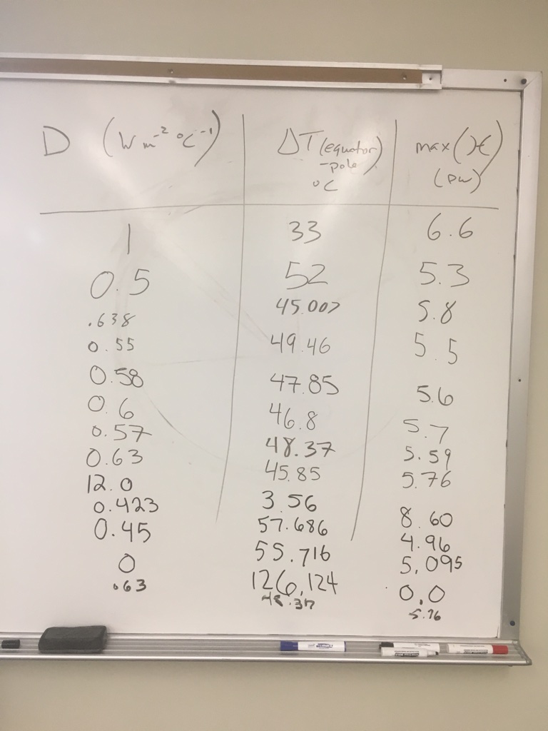
# ### Results
# 
# 12 students calculated $\Delta T$ and $\mathcal{H}_{max}$ for different values of the diffusivity parameter $D$. 
# 
# We collected the data on the whiteboard during class:

# ![column sketch](http://www.atmos.albany.edu/facstaff/brose/classes/ENV415_Spring2018/images/classdata.jpg)

# Here are the same data entered into a [Pandas data frame](http://pandas.pydata.org/pandas-docs/stable/10min.html).

# In[22]:


import pandas as pd
classdata = pd.DataFrame({'$D$': [1., 0.5, 0.638, 0.55, 0.58, 0.6, 0.57, 0.63, 12.0, 0.423, 0.45, 0., 0.63], 
                          '$\Delta T$': [33., 52., 45.007, 49.46, 47.85, 46.8, 48.37, 45.85, 3.56, 57.686, 55.716, 126.124, 48.37],
                          '$\mathcal{H}_{max}$': [6.6, 5.3, 5.8, 5.5, 5.6, 5.7, 5.59, 5.76, 8.60, 4.96, 5.095, 0., 5.76],
                         })
classdata


# Now we can do fun things like make a scatterplot of the data:

# In[23]:


fig, axes = plt.subplots(2,1)
classdata.plot.scatter(x='$D$', y='$\Delta T$', ax=axes[0])
classdata.plot.scatter(x='$D$', y='$\mathcal{H}_{max}$', ax=axes[1])


# Evidently the temperature gradient $\Delta T$ decreases with $D$, while the heat transport increases with $D$.

# ## A more systematic search

# In[24]:


Darray = np.arange(0., 2.05, 0.05)

model_list = []
Tmean_list = []
deltaT_list = []
Hmax_list = []

for D in Darray:
    ebm = climlab.EBM_annual(A=210, B=2, a0=0.354, a2=0.25, D=D)
    ebm.integrate_years(20., verbose=False)
    Tmean = ebm.global_mean_temperature()
    deltaT = np.max(ebm.Ts) - np.min(ebm.Ts)
    energy_in = np.squeeze(ebm.ASR - ebm.OLR)
    Htrans = ebm.heat_transport()
    Hmax = np.max(Htrans)
    model_list.append(ebm)
    Tmean_list.append(Tmean)
    deltaT_list.append(deltaT)
    Hmax_list.append(Hmax)


# In[34]:


color1 = 'b'
color2 = 'r'

fig, ax1 = plt.subplots(figsize=(8,6))
ax1.plot(Darray, deltaT_list, color=color1)
ax1.plot(Darray, Tmean_list, 'b--')
ax1.set_xlabel('D (W m$^{-2}$ K$^{-1}$)', fontsize=14)
ax1.set_xticks(np.arange(Darray[0], Darray[-1], 0.2))
ax1.set_ylabel('$\Delta T$ (equator to pole)', fontsize=14,  color=color1)
for tl in ax1.get_yticklabels():
    tl.set_color(color1)
ax2 = ax1.twinx()
ax2.plot(Darray, Hmax_list, color=color2)
ax2.set_ylabel('Maximum poleward heat transport (PW)', fontsize=14, color=color2)
for tl in ax2.get_yticklabels():
    tl.set_color(color2)
ax1.set_title('Effect of diffusivity on temperature gradient and heat transport in the EBM', fontsize=16)
#  Add our crowd-sourced data to the figure
classdata.plot.scatter(x='$D$', y='$\Delta T$', ax=ax1)
classdata.plot.scatter(x='$D$', y='$\mathcal{H}_{max}$', ax=ax2)
for ax in [ax1, ax2]:
    ax.set_xlim(0,2)
ax1.plot([0.6, 0.6], [0, 140], 'k-')
ax1.grid()


# When $D=0$, every latitude is in radiative equilibrium and the heat transport is zero. As we have already seen, this gives an equator-to-pole temperature gradient much too high.
# 
# When $D$ is **large**, the model is very efficient at moving heat poleward. The heat transport is large and the temperture gradient is weak.
# 
# The real climate seems to lie in a sweet spot in between these limits.
# 
# It looks like our fitting criteria are met reasonably well with $D=0.6$ W m$^{-2}$ K$^{-1}$

# Also, note that the **global mean temperature** (plotted in dashed blue) is completely insensitive to $D$. Why do you think this is so?

# ____________
# <a id='section7'></a>
# 
# ## 7. Summary: parameter values in the diffusive EBM
# ____________

# Our model is defined by the following equation
# 
# $$ C \frac{\partial T}{\partial t} = (1-\alpha) ~ Q - \left( A + B~T \right) + \frac{D}{\cos⁡\phi } \frac{\partial }{\partial \phi} \left(   \cos⁡\phi  ~ \frac{\partial T}{\partial \phi} \right) $$
# 
# with the albedo given by
# 
# $$ \alpha(\phi) = \alpha_0 + \alpha_2 P_2(\sin\phi) $$

# We have chosen the following parameter values, which seems to give a reasonable fit to the observed **annual mean temperature and energy budget**:
# 
# - $ A = 210 ~ \text{W m}^{-2}$
# - $ B = 2 ~ \text{W m}^{-2}~^\circ\text{C}^{-1} $
# - $ a_0 = 0.354$
# - $ a_2 = 0.25$
# - $ D = 0.6 ~ \text{W m}^{-2}~^\circ\text{C}^{-1} $

# In[ ]: