#!/usr/bin/env python
# coding: utf-8
# # Linear Classification
#
# - Algorithms that learn linear decision boundaries for classification tasks.
# - Note that the model can be non-linear such as logistic regression or SVM. But the decision boundary is linear.
# - The goal is to learn a hyper-plane $\mathbf{x}^T \mathbf{w} + b = 0$ to separate the date.
#
#  #
# ## Least square classification
#
# In assignment 1, we used linear regression for classification:
# $$y(\mathbf{x}, \mathbf{w}) = \mathbf{x}^T \mathbf{w} + b$$
#
#
#
# ## Least square classification
#
# In assignment 1, we used linear regression for classification:
# $$y(\mathbf{x}, \mathbf{w}) = \mathbf{x}^T \mathbf{w} + b$$
#
#  #
# ## Logistic Regression Model
#
# We will consider linear model for classification. Note that the model is linear in parameters.
#
# $$y(\mathbf{x}, \mathbf{w}) = \sigma (\mathbf{x}^T \mathbf{w} + b)$$
#
# where
#
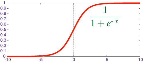
# $$ \sigma(x) = {1 \over {1 + e^{-x}}}$$
#
#
#
# ## Logistic Regression Model
#
# We will consider linear model for classification. Note that the model is linear in parameters.
#
# $$y(\mathbf{x}, \mathbf{w}) = \sigma (\mathbf{x}^T \mathbf{w} + b)$$
#
# where
#
# $$ \sigma(x) = {1 \over {1 + e^{-x}}}$$
#
#  # # Logistic Regression Example
# In[1]:
import tensorflow as tf
import numpy as np
import matplotlib.pyplot as plt
get_ipython().run_line_magic('pylab', 'inline')
import warnings
warnings.filterwarnings('ignore')
# ### Loading the dataset
# In[2]:
with np.load("TINY_MNIST.npz") as data:
x_train, t_train = data["x"], data["t"]
x_eval, t_eval = data["x_eval"], data["t_eval"]
# In[3]:
import nn_utils as nn
nn.show_images(x_train[:200], (10, 20), scale=1)
nn.show()
# ### Placeholders and Variables
# In[4]:
#Placeholders
X = tf.placeholder("float", shape=(None, 64))
Y = tf.placeholder("float", shape=(None, 1))
#Varialbels
W = tf.Variable(np.random.randn(64, 1).astype("float32"), name="weight")
b = tf.Variable(np.random.randn(1).astype("float32"), name="bias")
# In[5]:
X.get_shape()
# ### Logistic Regression Model
#
# We will consider linear model for classification. Note that the model is linear in parameters.
#
# $$y(\mathbf{x}, \mathbf{w}) = \sigma (\mathbf{x}^T \mathbf{w} + b)$$
# In[6]:
logits = tf.add(tf.matmul(X, W), b)
output = tf.nn.sigmoid(logits)
print output.get_shape()
# ## Cross-Entropy Cost
# Cross-Entropy cost = $t * -\text{log}(y) + (1 - t) * -\text{log}(1 - y)$
#
# Cross-Entropy cost = $t * -\text{log}(\sigma(x)) + (1 - t) * -\text{log}(1 - \sigma(x))$
#
# where $ \sigma(x) = {1 \over {1 + e^{-x}}}$
#
# ### Problem: This cost will give rise to NaN when $x \rightarrow -\infty, \infty$
# In[7]:
def sigmoid(x):
return 1.0 / (1.0 + np.exp(-x))
sigmoid(100)
# ### How not to do Cross Entropy
# In[27]:
#This doesn't work!
def xentropy(x, t):
return t*-np.log(sigmoid(x)) + (1-t)*-np.log(1.0 - sigmoid(x))
print xentropy(10, 1)
print xentropy(-1000, 0)
print xentropy(1000, 0)
print xentropy(-1000, 1)
# In[12]:
#This kind of works!
def hacky_xentropy(x, t):
return t*-np.log(1e-15 + sigmoid(x)) + (1-t)*-np.log(1e-15 + 1.0 - sigmoid(x))
print hacky_xentropy(1000, 1)
print hacky_xentropy(-1000, 0)
print hacky_xentropy(1000, 0)
print hacky_xentropy(-1000, 1)
# In[13]:
#This kind of works!
def another_hacky_xentropy(x, t):
return -np.log(t*sigmoid(x) + (1-t)*(1-sigmoid(x)))
print another_hacky_xentropy(1000, 1)
print another_hacky_xentropy(-1000, 0)
print another_hacky_xentropy(1000, 0)
print another_hacky_xentropy(-1000, 1)
# ### How to do Cross Entropy
# Cross-Entropy = $x - x * t + log(1 + e^{-x}) = max(x, 0) - x * t + log(1 + e^{-|x|}))$
# In[14]:
def good_xentropy(x, t):
return np.maximum(x, 0) - x * t + np.log(1 + np.exp(-np.abs(x)))
print good_xentropy(1000, 1)
print good_xentropy(-1000, 0)
print good_xentropy(1000, 0)
print good_xentropy(-1000, 1)
# In[15]:
x = np.arange(-10, 10, 0.1)
y = [good_xentropy(i, 1) for i in x]
plt.plot(x, y)
plt.grid(); plt.xlabel("logit"); plt.ylabel("Cross-Entropy")
# 1. Logistic Regression penalizes you linearly when you are on the wrong side of the hyperplane.
# 2. Logistic Regression doesn't penalizes you when you are on the right side of the hyper-plane but far away. (Not sensitive to outliers)
# 3. This is why we should use logistic regression instead of linear regression for classification (comes at the cost of not having a closed form solution).
# ## Support Vector Machines (SVM):
#
# - The logistic regression cost function is very similar to the cost function of SVM. SVM only considers the points that are close to the hyperplane (support vectors) and ignores the rest of the points:
# In[16]:
def svm_cost(x):
return - x + 1 if x < 1 else 0
x = np.arange(-10, 10, 0.1)
y = [svm_cost(i) for i in x]
plt.plot(x, y)
plt.grid(); plt.xlabel("logit"); plt.ylabel("Cross-Entropy")
# ## Cross Entropy in TensorFlow
# In[17]:
cost_batch = tf.nn.sigmoid_cross_entropy_with_logits(logits=logits, targets=Y)
cost = tf.reduce_mean(cost_batch)
# In[18]:
print logits.get_shape()
print cost.get_shape()
# In[19]:
norm_w = tf.nn.l2_loss(W)
# ## Momentum Optimizer
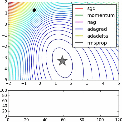
# "This is logistic regression on noisy moons dataset from sklearn which shows the smoothing effects of momentum based techniques (which also results in over shooting and correction). The error surface is visualized as an average over the whole dataset empirically, but the trajectories show the dynamics of minibatches on noisy data. The bottom chart is an accuracy plot." (Image by Alec Radford)
#
# 
# In[21]:
optimizer = tf.train.MomentumOptimizer(learning_rate=1.0, momentum=0.99)
# optimizer = tf.train.GradientDescentOptimizer(learning_rate=1.0)
train_op = optimizer.minimize(cost)
# ## Compute Accuracy
# In[22]:
#a hack for binary thresholding
pred = tf.greater(output, 0.5)
pred_float = tf.cast(pred, "float")
#accuracy
correct_prediction = tf.equal(pred_float, Y)
accuracy = tf.reduce_mean(tf.cast(correct_prediction, "float"))
# ## Creating a session
# In[23]:
sess = tf.InteractiveSession()
# ## Intitializing Variables
# In[24]:
init = tf.initialize_all_variables()
sess.run(init)
# ## Training
# In[25]:
for epoch in range(2000):
for i in xrange(8):
x_batch = x_train[i * 100: (i + 1) * 100]
y_batch = t_train[i * 100: (i + 1) * 100]
cost_np, _ = sess.run([cost, train_op],
feed_dict={X: x_batch, Y: y_batch})
#Display logs per epoch step
if epoch % 50 == 0:
cost_train, accuracy_train = sess.run([cost, accuracy],
feed_dict={X: x_train, Y: t_train})
cost_eval, accuracy_eval, norm_w_np = sess.run([cost, accuracy, norm_w],
feed_dict={X: x_eval, Y: t_eval})
print ("Epoch:%04d, cost=%0.9f, Train Accuracy=%0.4f, Eval Accuracy=%0.4f, Norm of Weights=%0.4f" %
(epoch+1, cost_train, accuracy_train, accuracy_eval, norm_w_np))
# ## $L_2$ Regularization
#
# As you can see when the data is linearly separable, the norm of W goes to infinity! (Can you explain why?)
#
# Add L2 regularization to the above code so as to prevent this from happening (only one line of code! Thanks to awesome TensorFlow!)
# # Non-Linear Feature Space
#
#
# # Logistic Regression Example
# In[1]:
import tensorflow as tf
import numpy as np
import matplotlib.pyplot as plt
get_ipython().run_line_magic('pylab', 'inline')
import warnings
warnings.filterwarnings('ignore')
# ### Loading the dataset
# In[2]:
with np.load("TINY_MNIST.npz") as data:
x_train, t_train = data["x"], data["t"]
x_eval, t_eval = data["x_eval"], data["t_eval"]
# In[3]:
import nn_utils as nn
nn.show_images(x_train[:200], (10, 20), scale=1)
nn.show()
# ### Placeholders and Variables
# In[4]:
#Placeholders
X = tf.placeholder("float", shape=(None, 64))
Y = tf.placeholder("float", shape=(None, 1))
#Varialbels
W = tf.Variable(np.random.randn(64, 1).astype("float32"), name="weight")
b = tf.Variable(np.random.randn(1).astype("float32"), name="bias")
# In[5]:
X.get_shape()
# ### Logistic Regression Model
#
# We will consider linear model for classification. Note that the model is linear in parameters.
#
# $$y(\mathbf{x}, \mathbf{w}) = \sigma (\mathbf{x}^T \mathbf{w} + b)$$
# In[6]:
logits = tf.add(tf.matmul(X, W), b)
output = tf.nn.sigmoid(logits)
print output.get_shape()
# ## Cross-Entropy Cost
# Cross-Entropy cost = $t * -\text{log}(y) + (1 - t) * -\text{log}(1 - y)$
#
# Cross-Entropy cost = $t * -\text{log}(\sigma(x)) + (1 - t) * -\text{log}(1 - \sigma(x))$
#
# where $ \sigma(x) = {1 \over {1 + e^{-x}}}$
#
# ### Problem: This cost will give rise to NaN when $x \rightarrow -\infty, \infty$
# In[7]:
def sigmoid(x):
return 1.0 / (1.0 + np.exp(-x))
sigmoid(100)
# ### How not to do Cross Entropy
# In[27]:
#This doesn't work!
def xentropy(x, t):
return t*-np.log(sigmoid(x)) + (1-t)*-np.log(1.0 - sigmoid(x))
print xentropy(10, 1)
print xentropy(-1000, 0)
print xentropy(1000, 0)
print xentropy(-1000, 1)
# In[12]:
#This kind of works!
def hacky_xentropy(x, t):
return t*-np.log(1e-15 + sigmoid(x)) + (1-t)*-np.log(1e-15 + 1.0 - sigmoid(x))
print hacky_xentropy(1000, 1)
print hacky_xentropy(-1000, 0)
print hacky_xentropy(1000, 0)
print hacky_xentropy(-1000, 1)
# In[13]:
#This kind of works!
def another_hacky_xentropy(x, t):
return -np.log(t*sigmoid(x) + (1-t)*(1-sigmoid(x)))
print another_hacky_xentropy(1000, 1)
print another_hacky_xentropy(-1000, 0)
print another_hacky_xentropy(1000, 0)
print another_hacky_xentropy(-1000, 1)
# ### How to do Cross Entropy
# Cross-Entropy = $x - x * t + log(1 + e^{-x}) = max(x, 0) - x * t + log(1 + e^{-|x|}))$
# In[14]:
def good_xentropy(x, t):
return np.maximum(x, 0) - x * t + np.log(1 + np.exp(-np.abs(x)))
print good_xentropy(1000, 1)
print good_xentropy(-1000, 0)
print good_xentropy(1000, 0)
print good_xentropy(-1000, 1)
# In[15]:
x = np.arange(-10, 10, 0.1)
y = [good_xentropy(i, 1) for i in x]
plt.plot(x, y)
plt.grid(); plt.xlabel("logit"); plt.ylabel("Cross-Entropy")
# 1. Logistic Regression penalizes you linearly when you are on the wrong side of the hyperplane.
# 2. Logistic Regression doesn't penalizes you when you are on the right side of the hyper-plane but far away. (Not sensitive to outliers)
# 3. This is why we should use logistic regression instead of linear regression for classification (comes at the cost of not having a closed form solution).
# ## Support Vector Machines (SVM):
#
# - The logistic regression cost function is very similar to the cost function of SVM. SVM only considers the points that are close to the hyperplane (support vectors) and ignores the rest of the points:
# In[16]:
def svm_cost(x):
return - x + 1 if x < 1 else 0
x = np.arange(-10, 10, 0.1)
y = [svm_cost(i) for i in x]
plt.plot(x, y)
plt.grid(); plt.xlabel("logit"); plt.ylabel("Cross-Entropy")
# ## Cross Entropy in TensorFlow
# In[17]:
cost_batch = tf.nn.sigmoid_cross_entropy_with_logits(logits=logits, targets=Y)
cost = tf.reduce_mean(cost_batch)
# In[18]:
print logits.get_shape()
print cost.get_shape()
# In[19]:
norm_w = tf.nn.l2_loss(W)
# ## Momentum Optimizer
# "This is logistic regression on noisy moons dataset from sklearn which shows the smoothing effects of momentum based techniques (which also results in over shooting and correction). The error surface is visualized as an average over the whole dataset empirically, but the trajectories show the dynamics of minibatches on noisy data. The bottom chart is an accuracy plot." (Image by Alec Radford)
#
# 
# In[21]:
optimizer = tf.train.MomentumOptimizer(learning_rate=1.0, momentum=0.99)
# optimizer = tf.train.GradientDescentOptimizer(learning_rate=1.0)
train_op = optimizer.minimize(cost)
# ## Compute Accuracy
# In[22]:
#a hack for binary thresholding
pred = tf.greater(output, 0.5)
pred_float = tf.cast(pred, "float")
#accuracy
correct_prediction = tf.equal(pred_float, Y)
accuracy = tf.reduce_mean(tf.cast(correct_prediction, "float"))
# ## Creating a session
# In[23]:
sess = tf.InteractiveSession()
# ## Intitializing Variables
# In[24]:
init = tf.initialize_all_variables()
sess.run(init)
# ## Training
# In[25]:
for epoch in range(2000):
for i in xrange(8):
x_batch = x_train[i * 100: (i + 1) * 100]
y_batch = t_train[i * 100: (i + 1) * 100]
cost_np, _ = sess.run([cost, train_op],
feed_dict={X: x_batch, Y: y_batch})
#Display logs per epoch step
if epoch % 50 == 0:
cost_train, accuracy_train = sess.run([cost, accuracy],
feed_dict={X: x_train, Y: t_train})
cost_eval, accuracy_eval, norm_w_np = sess.run([cost, accuracy, norm_w],
feed_dict={X: x_eval, Y: t_eval})
print ("Epoch:%04d, cost=%0.9f, Train Accuracy=%0.4f, Eval Accuracy=%0.4f, Norm of Weights=%0.4f" %
(epoch+1, cost_train, accuracy_train, accuracy_eval, norm_w_np))
# ## $L_2$ Regularization
#
# As you can see when the data is linearly separable, the norm of W goes to infinity! (Can you explain why?)
#
# Add L2 regularization to the above code so as to prevent this from happening (only one line of code! Thanks to awesome TensorFlow!)
# # Non-Linear Feature Space
#
#  #
#
#
# 