# # Historical high water levels of the river Ahr
#
# Topic: The purpose of this document is to provide some info about what was the situation that led to the "100-year" flood event of the river Ahr in Germany.
# In a follow up document we'll try to answer: "Why was the "100-year" flood event of the river Ahr in Germany on 14-15th July 2021 so catastrophic?"
# Author: Van Oproy Kurt
# ### Preliminary notes
# - The discharge values are the calculated daily or hourly averages, based on the water level measurement.
# - The datasets with hourly averages contain only data of the last 31 days.
# - The data and descriptions in historical records of similar floods had not been included in the top 10 high water dataset for making predictions.
# - The data which the RLP administration for environment used, had only a timespan going back 75 years. Or much less.
# - The rainfall amounts of 150-180 mm per day, which in some places occured in a few hours time, were predicted in time.
# - Some of the hydrometers broke down **before the peak flow**. One measurestation was completely washed away.
# - Some stations had direct communication links, but they broke down with the collapse of the telecom and electricity infrastructure.
# - So, the early warning system was partly cut down before the peak flow.
# - Nonetheless, I found 1 station that had all the values of the peak wave, so I'll try to construct a discharge curve of the composite water mass.
#
# ### References
# - Reconstructing peak discharges of historic floods of the river Ahr, Germany, 2014-01-05, Thomas Roggenkamp and Jürgen Herget
# - Ahr-Hochwasser am 12. 13. Juni 1910 forderte 52 Menschenleben, Leonhard Janta, Helmut Poppelreuter, Heimatjahrbuch Kreis Ahrweiler 2010
# - Ahrserie_Katastrophen_28_Juni_2014.pdf, NR. 139. MITTWOCH 18 JUNI 2014, Rhein-Zeitung Epaper - Mittelrhein-Verlag, Koblenz,Germany, Petra Ochs
# - Die Ahr und ihre Hochwässer in alten Quellen. Karl August Seel, Heimatjahrbuch des Kreises Ahrweiler 40, 1983
# - Das Hochwasser von 1804 im Kreise Ahrweiler, Dr. Hans FRICK, [hjb1955](https://kreis-ahrweiler.de/kvar/VT/hjb1955/hjb1955.11.htm)
# - This was an update of his original publication from 1929.
# - Das Naturschutzgebiet Ahrschleife bei Altenahr, Teil 2, Büchs, W.
# - Floods in Germany - Analyses of Trends, T. Petrow: Dr. diss.
# - Characteristics and process controls of statistical flood moments in Europe – a data based analysis, 2020, David Lun, Alberto Viglione, Miriam Bertola, Jürgen Komma, Juraj Parajka1, Peter Valent, Günter Blöschl, https://doi.org/10.5194/hess-2020-600
# - [RLP administration for environment](https://geoportal-wasser.rlp-umwelt.de/servlet/is/2025/)
#
# ### Post-flood event references
# - Hochwasser Mitteleuropa, Juli 2021 (Deutschland), CEDIM Forensic Disaster Analysis (FDA) Group, 21. Juli 2021 – Bericht Nr. 1 "Nordrhein-Westfalen & Rheinland-Pfalz"
# - [Déjà-vu der Katastrophe](https://www.faz.net/aktuell/wissen/erde-klima/flutkatastrophe-im-ahrtal-neue-erkenntnisse-zum-hochwasser-17470847.html), OLIVER SCHLÖMER, JENS GIESEL und MANFRED LINDINGER · 5. August 2021
# - Katastrophale Hochwasser im Ahrtal 2021, 1910, 1804, 1719 und 1601, [reitschuster.de](https://reitschuster.de/post/katastrophale-hochwasser-im-ahrtal-2021-1910-1804-1719-und-1601/)
# ##### Slope of the steep hill at Dernau
# In[28]:
(300-160)/518
import this
# In[2]:
import numpy as np
import matplotlib.pyplot as plt
import seaborn as sns
import pandas as pd
sns.set()
sns.set_context('notebook')
np.set_printoptions(threshold=20, precision=2, suppress=True)
pd.options.display.max_rows = 57
pd.options.display.max_columns = 38
pd.set_option('precision', 2)
from IPython.display import Image, display
get_ipython().run_line_magic('config', "InlineBackend.figure_format = 'retina'")
from IPython.core.display import display, HTML
display(HTML(""))
# In[3]:
get_ipython().run_line_magic('autosave', '400')
# In[3]:
Ahr =pd.read_csv(r"Ahr Aktuelle Wasserstände.csv",sep="\t", skiprows=2,usecols=[1,2],index_col=0,na_values= "-"); # header=0,sep=\";\",\n",
Ahr.index = pd.to_datetime(Ahr.index, format="%d.%m.%Y %H:%M") # parse_dates=["Datum"]
Abfluss =pd.read_csv(r"Ahr Abfluss.csv",sep="\t", index_col=1,na_values= "-",decimal=","); #parse_dates=["Datum"],
Abfluss.index = pd.to_datetime(Abfluss.index, format="%d.%m.%Y %H:%M")
Ahr.head(10)
# ## Pegel Altenahr
# In[42]:
Ahr.info()
# In[42]:
Ahrstats =pd.read_csv(r"Ahr.csv", skiprows=2,sep="\t",index_col=0,decimal="," ,);
Hochwasser =pd.read_csv(r"AhrHochwasserereignisse19462019.csv",parse_dates=["Datum"],skiprows=2,sep="\t",index_col=1,decimal=",",
engine='python'); #skipfooter=1
#floods[\"Date\"] = pd.to_datetime( River_Arno.Date, format='%d/%m/%Y' ) # euro dates\n",
#floods.set_index(\"Date\", inplace=True)\n",
Ahrstats.head(10)
# Since the calibration curve for the high water levels to estimate the interval of a "100 year flood" is actually based on a shorter period, in fact 1946-2019, we have to correct the timespan accordingly...
# In[78]:
Ahrstats["days"]=Ahrstats.index*365
#Ahrstats["year"]= Ahrstats.Jährlichkeiten
Ahrstats["years"]= Ahrstats.index*((2021.5 -1946)/100)
# In[79]:
Ahrstats.head(11)
# ## Precipitation data
# ### Daily Barweiler
# In[8]:
Barweiler =pd.read_csv(r"stundenwerte_RR_03660_akt\produkt_rr_stunde_20200130_20210801_03660.txt",sep=";",index_col=1,
na_values= "-999",); # header=0,sep=\";\",\n", ,usecols=[2,3], parse_dates=["MESS_DATUM"]
Barweiler.index = pd.to_datetime(Barweiler.index, format="%Y%m%d%H") # -%M-
Barweiler.head(10)
# In[8]:
Barweiler.tail(3)
# In[30]:
Barweiler[" R1"].plot();
# In[42]:
Barweiler["2021-07-07":"2021-07-16"][" R1"].plot();
# In[31]:
Barweiler.info()
# In[34]:
Barweiler[" R1"].resample("D").sum().plot();
# In[38]:
BarweilerD= Barweiler[" R1"].resample("D").sum()
BarweilerD.rolling(7).sum().plot();
# In[39]:
BarweilerD.rolling(14).sum().plot();
# ### Daily Adenauer
# In[46]:
Adenauer =pd.read_csv(r"stundenwerte_RR_03490_akt\produkt_rr_stunde_20200130_20210715_03490.txt",sep=";",index_col=1,
na_values= "-999",); # header=0,sep=\";\",\n", ,usecols=[2,3], parse_dates=["MESS_DATUM"]
Adenauer.index = pd.to_datetime(Adenauer.index, format="%Y%m%d%H") # -%M-
Adenauer.head(10)
# In[47]:
Adenauer.tail(10)
# In[43]:
Adenauer["2021-07-07":"2021-07-16"][" R1"].plot();
# In[48]:
Adenauer.info()
# In[49]:
AdenauerD= Adenauer.iloc[:,2].resample("D").sum()
BarweilerD= Barweiler.iloc[:,2].resample("D").sum()
BarweilerD["2021-07-01":"2021-07-16"].plot();
# In[50]:
AdenauerD["2021-07-01":"2021-07-16"].plot();
# In[52]:
AhrD= Ahr.iloc[:,0].resample("D").sum()/24
AhrD.loc["2021-07-01":"2021-07-16"].plot();
# In[53]:
AhrD.loc["2021-07-01":"2021-07-16"]
# In[54]:
AhrH= Ahr.iloc[:,0]#.resample("H").mean()
AhrH.loc["2021-07-01":"2021-07-16"].plot();
# In[41]:
Ahr.loc["2021-07-01":"2021-07-16"].plot();
# Müsch has 352 km² drainage area, and suppose 100 liter fell in 2 days time:
# In[46]:
100*1000*1000/1000*352/(3600*24)
# >3500 m³ on 2days time needs a discharge of 400 cum/sec.
# Datum Abfluss in m3/s Abflussspende in L/(s*km2) Wasserstand in cm
# 02.06.2016 132 374 273
# In[47]:
170*1000*1000/1000*352/(3600*24)
# In[ ]:
# ### Soil moisture content
# Water content in the upper soil layers 10 cm thick, up till 60 cm deep.
# In[9]:
soil =pd.read_csv(r"derived_germany_soil_daily_recent_3660.txt\derived_germany__soil__daily__recent__3660.txt",sep=";",index_col=1,
na_values= "-999",); # header=0,sep=\";\",\n", ,usecols=[2,3], parse_dates=["MESS_DATUM"]
soil.index = pd.to_datetime(soil.index, format="%Y%m%d") # -%M-
soil.loc["July 2021"].head(16)
# In[10]:
soilmoisture= soil[["BF10" ,"BF20","BF30","BF40","BF50","BF60"]]
soilmoisture60= soil[["BF60"]]
# In[11]:
soilmoisture["BFSUM"]= soilmoisture["BF10"]+soilmoisture["BF20"]+soilmoisture["BF30"]+soilmoisture["BF40"]+soilmoisture["BF50"]+soilmoisture["BF60"]
# In[51]:
soilmoisture60.plot( figsize=(16,5), grid=True, title="soil moisture under grass and sandy loam between 0 and 60 cm depth in % plant useable water"); # .loc["28 June 2021":"18 July 2021"]
# In[15]:
soilmoisture["BFSUM"].plot( figsize=(16,5), grid=True, title="soil moisture under grass and sandy loam between 0 and 60 cm depth in % plant useable water"); # .loc["28 June 2021":"18 July 2021"]
# In[19]:
soilmoisture["BFSUM"].max()
# The soil was at 13-07-2021 up till 60 cm deep full of water.
# In[20]:
soilmoisture.loc["28 June 2021":"18 July 2021"].plot( figsize=(16,5), grid=True, title="soil moisture under \
grass and sandy loam between 0 and 60 cm depth in % plant useable water");
# In[12]:
soilhistor =pd.read_csv(r"derived_germany_soil_daily_historical_3660.txt\derived_germany__soil__daily__historical__3660.txt.csv",sep=";",index_col=1,
na_values= "-999",); # header=0,sep=\";\",\n", ,usecols=[2,3], parse_dates=["MESS_DATUM"]
soilhistor.index = pd.to_datetime(soilhistor.index, format="%Y%m%d") # -%M-
soilhistor.head(16)
# In[13]:
soilmoisturehistor= soilhistor[["BF10" ,"BF20","BF30","BF40","BF50","BF60"]]
soilmoisturehistor["BFSUM"]= soilhistor["BF10"]+soilhistor["BF20"]+soilhistor["BF30"]+soilhistor["BF40"]+soilhistor["BF50"]+soilhistor["BF60"]
soilmoisturehistor40= soilhistor["BF10"]+soilhistor["BF20"]+soilhistor["BF30"]+soilhistor["BF40"]
soilmoisturehistor30= soilhistor["BF10"]+soilhistor["BF20"]+soilhistor["BF30"]
# In[9]:
soilmoisturehistor.plot( figsize=(21,5), grid=True, title="historical soil moisture under \
grass and sandy loam between 0 and 60 cm depth in % plant useable water");
# In[68]:
soilmoisturehistor["2015":].plot( figsize=(21,5), grid=True, title="historical soil moisture under \
grass and sandy loam between 0 and 60 cm depth in % plant useable water");
# In[17]:
soilmoisturehistor["BFSUM"].plot( figsize=(16,5), grid=True, title="soil moisture under grass and sandy loam between 0 and 60 cm depth in % plant useable water"); # .loc["28 June 2021":"18 July 2021"]
# In[18]:
soilmoisturehistor["BFSUM"].max()
# In[73]:
soilmoisturehistor30["2015":].plot( figsize=(16,5), grid=True, title="historic soil moisture under grass and sandy loam between 0 and 30 cm depth in % plant useable water"); # .loc["28 June 2021":"18 July 2021"]
# In[15]:
soilmoisturehistorBFSUM =soilmoisturehistor["BFSUM"] # normalize only bfsum
soilmoistureBFSUM =soilmoisture["BFSUM"]
# In[67]:
sns.histplot( data=soilmoisturehistorBFSUM, kde=True, common_norm=True,cumulative=True, stat="probability", )
sns.histplot( data=soilmoistureBFSUM, kde=True, common_norm=True, cumulative=True, stat="probability",color='darkorange');
# The moisture content in the soil was throughout 2021 above average.
# In[34]:
soilmoistureBFSUM["2021-07-13":"2021-07-16"]
# For comparison: the situation of the soil moisture content during the flood of 2016-02-06. The total value for 2016 is 663 % for the 6 layers, compared to 732 % for the 2021 flood.
# The cause of this great difference were the biblical rainfall amounts of 2021 and slow moving clouds.
# Anyway I think this is a good indicator for acuteness of the situation.
# In[14]:
soilmoisturehistor.loc["2016-01-01": "2016-02-21"].iloc[:,:6].plot();
# In[19]:
soilmoisturehistorBFSUM.loc["2016-01-01": "2016-02-21"].plot(); # .iloc[:,:6]
# In[38]:
fig, ax=plt.subplots(figsize=(18,5));
soilmoisturehistorBFSUM.loc["2010-01-01": "2021-02-21"].plot(figsize=(18,5), grid=True,ax=ax, cmap='tab20b'); # .iloc[:,:6]
ax.axhline(y=730,linestyle ='--',color="red");
ax.axhline(y=655,linestyle =':',color="orange");
# ### The soil moisture content vs. water level of river Ahr
# The higher the soil moisture content of the upper layers is, the sooner rainfall will reach the runoff point, when any rainfall just runs off the slope.
# In[35]:
AhrDMax= Ahr.iloc[:,0].resample("D").mean()
# In[36]:
soilmoisture_pegel = pd.merge( soilmoistureBFSUM, AhrDMax, left_index=True,right_index=True, )
soilmoisture_pegel
# In[37]:
soilmoisture_pegel.plot(figsize=(14,5), grid=True, kind="bar");
# ### Yearly rainfall maxima
# In[33]:
klima_jahr_1930 =pd.read_csv(r"jahreswerte_KL_03490_19300101_20191231_hist\produkt_klima_jahr_19300101_20191231_03490.txt",sep=";",index_col=1,
na_values= "-999",); # header=0,sep=\";\",\n", ,usecols=[2,3], parse_dates=["MESS_DATUM"]
klima_jahr_1930.index = pd.to_datetime(klima_jahr_1930.index, format="%Y%m%d") # -%M- MESS_DATUM_BEGINN
klima_jahr_1930.head()
# In[48]:
klima_jahr_1930.tail()
# In[47]:
sns.lineplot( data=klima_jahr_1930.JA_MX_RS, );
# In[42]:
sns.histplot( data=klima_jahr_1930.JA_MX_RS, bins=20, kde=True);
# Pretty remarkable that the historical dataset for yearly maxima has no value above 70 mm/day. On the other hand there were values around 170 mm/day for the day of the big flood.
# In[45]:
from reliability.Distributions import Weibull_Distribution
from reliability.Probability_plotting import Weibull_probability_plot
import matplotlib.pyplot as plt
from reliability.Other_functions import make_right_censored_data
#dist = Exponential_Distribution(Lambda=0.25, gamma=12)
raw_data =klima_jahr_1930.JA_MX_RS.dropna() # dist.random_samples(100, seed=42)draw some random data from an exponential distributio
raw_data =raw_data.values
#data = make_right_censored_data(raw_data, threshold=17) # right censor the data at 17
Weibull_Distribution(alpha=20,beta=2, gamma=5 ).CDF(linestyle='--', label='True CDF') # we can't plot dist because it will be location shifted
Weibull_probability_plot(failures=raw_data, fit_gamma=True) # do the probability plot. Note that we have specified to fit gamma
plt.legend()
plt.show()
# Highwater marks on an old house in Dernau. Source: Dirk Sebastian
#
# ## High water level events of the Ahr
# It is actually easy to find many sources with good information online: *google "hochwasser der Ahr"*
# - Beim Hochwasser am 21. Juli 1804 starben 64 Menschen. Beim Hochwasser am 13. Juni 1910 starben 57 *(or 150?)* Menschen;[9] danach mussten alle Ahr-Brücken – außer der bei Rech – wiederaufgebaut werden. Im Ahrstraßentunnel in Altenahr sind Marken der höchsten Pegel angebracht.
#
# - Am 2. Juni 2016 erreichte der Pegel der Ahr in Kreuzberg und Altenahr seinen seit Messbeginn bis dahin höchsten Stand. Am Pegel Altenahr stieg die Ahr auf 369 Zentimeter, 20 cm mehr als beim zuvor höchsten Hochwasser 1993.[10]
#
# - Im Laufe des 14. Juli 2021 führten starke und anhaltende Regenfälle zu den bisher höchsten Pegelständen, die jemals gemessen wurden. Die Messstation in Altenahr gab um 20:45 Uhr einen Pegelstand von 575 cm an[11] und in Bad Bodendorf am 15. Juli 2021 um 03:45 Uhr einen Stand von 483 cm.[12] Am 14. Juli 2021 erreichte der Pegel Altenahr einen Wasserstand von etwa 700 cm.[13] Somit wurden die Pegelstände des „Jahrhunderthochwassers“[14] von 2016 um rund 3,3 Meter übertroffen.
#
# - Heimatforscher Dr. Hans Frick, der das Hochwasser von 1804 im Jahre 1929 als Erster umfassend darstellte: Jede Vorsorge war nutzlos, denn so hoch hatte die Ahr bis dahin noch nie gestanden. Über der Steinbrücke bei Rech soll sie eine Höhe von acht Fuß (etwa 2,50 Meter) erreicht haben... Fast alle Ahrbrücken – einer Aufstellung nach 30 Stück – stürzten ein, auch die aus Stein. Nach der gleichen Quelle verschwand auch der 18 Fuß (5,50 Meter) über normalem Wasserstand der Ahr gelegene Stotzheimer Hof bei Rech spurlos.
#
# Dr. Hans Frick was the first geographer who searched for historical source materials which dated more than 100 years ago.
# Here are translations of some of the old texts, and citation from Hr. Seel: „Die Ahr und ihre Hochwässer in alten Quellen“ :
#
# - On May 30th 1601, “what day has been the Lord's Ascension evening”, the sky darkened in the afternoon, according to the chronicle from the village of Antweiler. A "thunderstorm" with rain and hail "fell down" so forceful that the residents believed in the end of the world. The subsequent flood "suffered other great damage with 16 buildings, houses, sheds and places and 9 people drowned." In a village in which only about 180 souls lived at that time.
#
# - The Antweiler Chronicle **does not report how great the damage was further downstream** in Anno Domini 1601. But one can assume that they were also considerable, because Antweiler is located on the upper reaches of the Ahr and the tidal wave of the "storm" flowed further downstream, then as now. About ten kilometers away in the village of Schuld, which was hit particularly hard by the floods last week. *The similarity with the build up and the damage of the 2021 flood is striking.*
#
# - Tuesday, August 1, 1719. This time too, the Ahr emerged from its river bed. Not as devastating as 118 years ago but with power. The chronicle of the monastery on Kalvarienberg in today's Bad Neuenahr-Ahrweiler reports that a wall in Heppingen was simply "overturned" by the flood, as was an avenue whose posts were "driven as far as Lorsdorf", i.e. about two current kilometers by car downstream. Two servants and an administrator of the monastery had only been able to save themselves in the trees until "help" came. The water had come so quickly.
# - The flood had also caused damage to the upper reaches of the Ahr, for example the village chapel in Schuld, which had only been built 20 years earlier, had to be completely renovated.
#
#
# - July 21, 1804: According to reports from the French authorities responsible at the time, the Ahr had been flooding for days when a storm followed on July 21. Within a short time all tributaries swelled up. Then the tide came. In today's Bad Neuenahr-Ahrweiler a chronicler wrote that the whole "getraidt was flooded". And Pastor Fey in Bodendorf, six kilometers downriver, noted in his diary: 'On July 21st, I went with Herr[n] Dean Radermacher over the mountain to Remagen [on the Rhine] and it started to rain this hard on top of the mountain so that we both arrived in Remagen soaked to the skin. In the same night the Ahr grew so much that ... all possible household utensils, timber and dead people were found in the field who had been driven there with the Ahr.'
#
# - Fields washed away down to the rock.
#
# - A plaque in the community center of Dorsel on the upper reaches of the Ahr still reminds of the devastating flood of 1804: “21. Julius at 3 o'clock in the afternoon, during a terrible thunderstorm coming from the north, the water fell in streams from the clouds, causing the bottom to flow from many fields to the rocks ... [and] the steel foundry suddenly "wiped out". The water covered "large masses of earth, sand, hedges and shrubs" and also tore away the "very strong stone foundry bridge".
#
# - The only reminder of the Dorsel steel foundry, to which the bridge belonged, is the campsite of the same name.
#
# - A total of 63 people were killed in the disaster. The same happened to many horses, draft cattle and feeder cattle. A total of 129 houses, 162 barns and stables, 18 mills, eight blacksmiths and almost all bridges were destroyed. Another 469 houses, 234 barns and stables, two mills and a forge were damaged. Churches and houses were almost without exception under water. Fruit trees were uprooted, vineyards washed away, the harvest destroyed and the meadows of the floodplains silted up with gravel and rubble.
#
# ### The top 10 high water events 1946 - 2019
# ... to which I added the estimated, sts. calculated, values of some historical flood events.
# In[43]:
Hochwasser= Hochwasser.sort_index( ascending=True)
Hochwasser.head(19)
a provisional estimation of the drainage area:if Hochwasser.iloc[:,2]!= np.nan :
Hochwasser["km2"]= Hochwasser.iloc[:,1]/Hochwasser.iloc[:,2]*1000
elif Hochwasser.iloc[:,2]!= "" :
Hochwasser["km2"]= Hochwasser.iloc[:,1]/Hochwasser.iloc[:,2]*1000
else:
Hochwasser["km2"]= np.nanHochwasser2= Hochwasser.iloc[:,2].astype('Int64')
Hochwasser1 =Hochwasser.iloc[:,1].astype('Int64') #Hochwasser1 /
Hochwasserlist =[Hochwasser1/int(x)*1000 for x in Hochwasser2 if x != np.nan if x != "" ]
Hochwasserlist
# ["km2"]else np.nan
# elif Hochwasser.iloc[:,2]!= "" : Hochwasser["km2"]= Hochwasser.iloc[:,1]/Hochwasser.iloc[:,2]*1000
#else: Hochwasser["km2"]=type(Hochwasserlist)type(Hochwasserlist[0])Hochwasser["km2"]=Hochwasserlist[0]
# Hochwasser2021= Hochwasser[~Hochwasser.iloc[6,:] ] #Hochwasser= "1993-12-01"
# Hochwasser2021
# In[45]:
Hochwasser.iloc[6,:]
# In[46]:
Hochwasser.info()
# In[47]:
Hochwasser[Hochwasser["Nr."]==14]
# - the former lowest value in the official list of top 10 HW events should go as I inserted the 2021 event
# - calculate the time interval between the events of flooding > recurrence interval
# In[48]:
Hochwasser["year"]= Hochwasser.index.year
Hochwasser["years"]=2021.5- Hochwasser["year"] # avoid 0
import datetime
today = datetime.date.today()
Hochwasser["days"]= (pd.to_datetime(today) - Hochwasser.index).days
import datetime
today = datetime.date.today()
dt= pd.to_datetime('1910/06/13', format='%Y/%m/%d') # date of earlier big flood 1946/08/01
Timesbetween= []
for ind in Hochwasser.index:
dt1= ind
print( dt1)
interval= (dt1-dt).days
print( interval)
#Timesbetween= Timesbetween+ list(interval)
dt =dt1
print( pd.to_datetime(today), (pd.to_datetime(today) -ind).days)
#Timesbetween
# In[246]:
pd.to_datetime('1910/06/13', format='%Y/%m/%d')-pd.to_datetime('2021/07/26', format='%Y/%m/%d')
intervals={"1910-06-13 00:00:00":40586,
"1961-01-31 00:00:00":5297,
"1966-11-12 00:00:00":2111,
"1984-05-30 00:00:00":6409,
"1984-07-02 00:00:00":33,
"1984-11-23 00:00:00":144,
"1988-03-16 00:00:00":1209,
"1993-12-21 00:00:00":2106, # the former lowest val should go as I inserted the 2021 event
"1995-01-23 00:00:00":398,
#"1993-12-21 00:00:00":20,
"2016-02-06 00:00:00":7684,
"2021-07-14 00:00:00":1985}
intervals= pd.DataFrame.from_dict(intervals, orient='index',columns=['TimeInterval']) #index= intervals[0]
type(intervals)intervals.plot();intervals.info()int10= intervals.index
int10
# In[50]:
fig,ax=plt.subplots( 1,1, figsize=(12,5))
sns.scatterplot(x=Hochwasser["Abfluss in m3/s"] ,y=Hochwasser.years, data=Hochwasser,hue=Hochwasser["year"],palette="magma")#hue=int10 [:-1]
plt.xscale("log") #ax.xaxis_scale("log")
# In[51]:
fig,ax=plt.subplots( 1,1, figsize=(12,6))
sns.scatterplot(x=Hochwasser["years"] ,y=Hochwasser["Wasserstand in cm"].values, data=Hochwasser,hue=Hochwasser["year"],palette="magma")#hue=int10
plt.xscale("log") #ax.xaxis_scale("log")
plt.legend() ;
#
# Highwater marks on the Ahrbrücke in Altenahr
#
# In[52]:
Hochwasser["Wasserstand in cm"]
# In[53]:
Hochwasser
# A small correction to avoid a log error because of a year with value 0: let's assume that 2021 was a 100 year flood event
# In[21]:
# small correction to avoid log error for a year with value 0: a 100 year flood event
Hochwasser.loc[Hochwasser["Nr."]==11, "years"]=100
# In[54]:
Hochwasser
# In[72]:
fig,ax=plt.subplots( 1,1, figsize=(9,6))
sns.regplot(x=Hochwasser["years"] ,y=Hochwasser["Wasserstand in cm"].values, data=Hochwasser,order=3, ci=67);#logx=True,
#plt.xscale("log") #ax.xaxis_scale("log")
plt.ylim(0,);
# The 2 waterlevels for 1804 have been described for the locations Rech and Altenahr.
# In[62]:
Hochwasser_exc2021= Hochwasser.loc["1800":"2020"]; Hochwasser_exc2021
# In[74]:
fig,ax=plt.subplots( 1,1, figsize=(9,6))
sns.regplot(x=Hochwasser["years"] ,y=Hochwasser["Abfluss in m3/s"].values, data=Hochwasser_exc2021,logx=True,truncate=True);#[:-2]hue=int10
plt.ylim(0,); #plt.xscale("log") #ax.xaxis_scale("log")
# In[75]:
fig,ax=plt.subplots( 1,1, figsize=(9,6))
sns.regplot(x=Hochwasser["years"] ,y=Hochwasser["Abfluss in m3/s"].values, data=Hochwasser_exc2021,order=1,truncate=True);#[:-2]hue=int10
plt.ylim(0,); #plt.xscale("log") #ax.xaxis_scale("log")
# ### The effect of applying a short time range for historical data.
# I made an interval curve based on historical sources, versus the official interval curve based on 'instrumental data'.
# In[77]:
Ahrstats
# In[85]:
fig,ax=plt.subplots(1,1, figsize=(16,7),sharey=True) #
#sns.regplot(x=Hochwasser.iloc[[0,14,11,12,13,15,16],: ].years ,y=Hochwasser.iloc[[0,14,11,12,13,15,16],: ]["Abfluss in m3/s"].values, #"Abfluss in m3/s"
# data=Hochwasser.iloc[[0,14,11,12,13,15,16],: ], logx=True, ci=95,truncate=True,ax=ax[0],label="Based on historical sources")#[1:-1]hue=int10 days.values
#sns.regplot(x=Hochwasser[1:11].years ,y=Hochwasser[1:11]["Abfluss in m3/s"].values, data=Hochwasser[1:11],logx=True, ci=95,ax=ax[0],label="Based on 'instrumental data'")
plt.ylabel("Discharge in m3/s")
sns.regplot(x=Ahrstats.years.values ,y=Ahrstats["Abfluss [m³/s]"].values,color="darkorange", data=Ahrstats,logx=True, ci=95,ax=ax, label="Top 10 data starting 1946")#hue=int10
sns.regplot(x=Hochwasser_exc2021.years ,y=Hochwasser_exc2021["Abfluss in m3/s"].values,
data=Hochwasser_exc2021, logx=True, ci=95,truncate=True,ax=ax, label="Top 17 data starting 1800")
plt.ylim(0,1250) #ax.xaxis_scale("log")
plt.legend()
plt.title("Top 15 data starting 1800 vs Discharge in m3/s");
# In[79]:
Hochwasser.iloc[[0,14,11,12,13],: ].year
# The highwater curve is merely based on data from 1946-2016. The timeline of that dataset was not large enough to be able to predict a flooding the size of 2021. However, there are high water level markings left from the horrible flood of June 1911, and the insane massive flood of 1804.
# The 3rd highest flood level was reached in 1601, according authors before the flood of 2016.
#
# *„30. May 1601, Antweiler: An diesem Tag erhob sich unversehens am Nachmittag ein Ungewitter mit Regen und Hagel, verfinsterte sich der Himmel, die Schleusen des Himmels öffneten sich und unvorstellbare Wassermassen stürzten hernieder, so daß die entsetzten Bewohner an den Weltuntergang glaubten“
# in SEEL: „Die Ahr und ihre Hochwässer in alten Quellen“*
#
# The streettunnel in Altenahr was only build in the 1830's, so the flood of 1804 could not make a bypass at that point. In 1910 the flood did exactly that, and reached a height in the tunnel of 2 meters. This tunnel has been made a bit more high and wide later on.
#
# Estimation of altitude of the streettunnel in AltenAhr: it is located about 6.5 meter above the average level of the Ahr. Considering a water level of +- 2 meter in the tunnel, and the formation of some bulging of the water front by about 25-50 cm, I come to a water level of about 850 mm or more. This value is based on the recent water level calibration.
# In[47]:
Ahrstats['Abfluss [m³/s]'].plot();
# In[107]:
Ahrstats.columns
#
#
# Stonebridge destroyed in Mayschoss, 1910
#
# In[27]:
print( "hydr. radius", 8.5*4/(4+8.5+4), (8.25*2.25+6.25*2.25)*4)
# In[31]:
R=8.5*4/(4+8.5+4)
S=0.005
n=0.033
V= R**(2/3)*(S**0.5)/n
V
# The velocity of water flowing in a stream or open channel is affected by a number of factors.
# In[30]:
R=8.5*4/(4+8.5+4)
S=0.005
n=0.15 # very overgrown
V= R**(2/3)*(S**0.5)/n
V
# ### The rate by which the flood rose on 2021-07-14.
# The hydrometers were positioned in order to be able to survive a "100 year flood" event, which was in fact based on a poor dataset. Eventually the hydrometers failed on 14 July, because they were placed to withstand floods not higher than 3 meters above the "average high water extreme". *This is only a translation from the German text on wasserportal.rlp-umwelt.de.*
# In[65]:
Ahr["2021-07-13":"2021-07-14"].plot(figsize=(16,5));
# Abflussspende, Wassermenge in Liter pro Sekunde, die in einem Einzugsgebiet bezogen auf eine Einheitsfläche von 1 km² abfließt.
# In[84]:
fig,ax=plt.subplots( 1,1, figsize=(16,5))
sns.scatterplot(data=Abfluss.iloc[:,1 ]["2021-07-14"])
sns.lineplot( data=Ahr.iloc[:,0 ]["2021-07-14"],color="crimson", ax=ax);
# Exclusive photo of the tunnels in Altenahr in the morning of 15 07 2021. It was taken by alerted inhabitants who left to warn family members in Altenahr, because they could not reach them by phone. They had to spent the night in the hills, and were probably the first "rescuers" in Altenahr.
#
# ### Discharge vs. waterlevel for Altenahr
# Here we combine recent and historical waterlevels together with the discharges calculated by various authors.
# In[88]:
fig,ax=plt.subplots( 1,1, figsize=(16,5))
plt.title("Discharge vs. waterlevel for Altenahr")
sns.scatterplot(x=Abfluss["2021-07-14"]["Abfluss in m3/s"], y=Ahr["2021-07-14"]["Wasserstand in cm"], data=Abfluss["2021-07-14"], label="pegel 2021-07-14");
sns.scatterplot(x=Hochwasser.iloc[:,1], y=Hochwasser.iloc[:,3], data=Hochwasser,hue=Hochwasser.index.date,palette="magma",); #**{marker.edgecolor:"indigo"}
# The difference between the series can be caused by human measurements in the past, a different river profile, sediment removal, or flood deposits. In fact there was in 2021 at least 1 bridge which watergates were completely clogged by a mix of debris: cars, wood logs, trees...
#
# This Image by Roggenkamp T. and co. Herget lays bare the drama of the fall out of the hydrometers. I guess the peak in Altenahr arrived at or just after midnight. These authors say that the tributary Sahrbach had a big impact on the pegel in Altenahr, so I take a look at the public available measure station there: Kreuzberg. [source: ](https://www.faz.net/aktuell/wissen/erde-klima/flutkatastrophe-im-ahrtal-neue-erkenntnisse-zum-hochwasser-17470847.html)
# ### Estimated parameters of the 1910 flood in Bad Neuenahr
# In[59]:
flood1910= pd.read_excel(r"Ahr2.xlsx", skiprows=1,engine="openpyxl",index_col=0,na_values= "", sheet_name="flood_1910")
flood1910T= flood1910.iloc[:,:4].T
flood1910T
# In[63]:
sns.scatterplot( data=flood1910T ,)
plt.yscale("log")
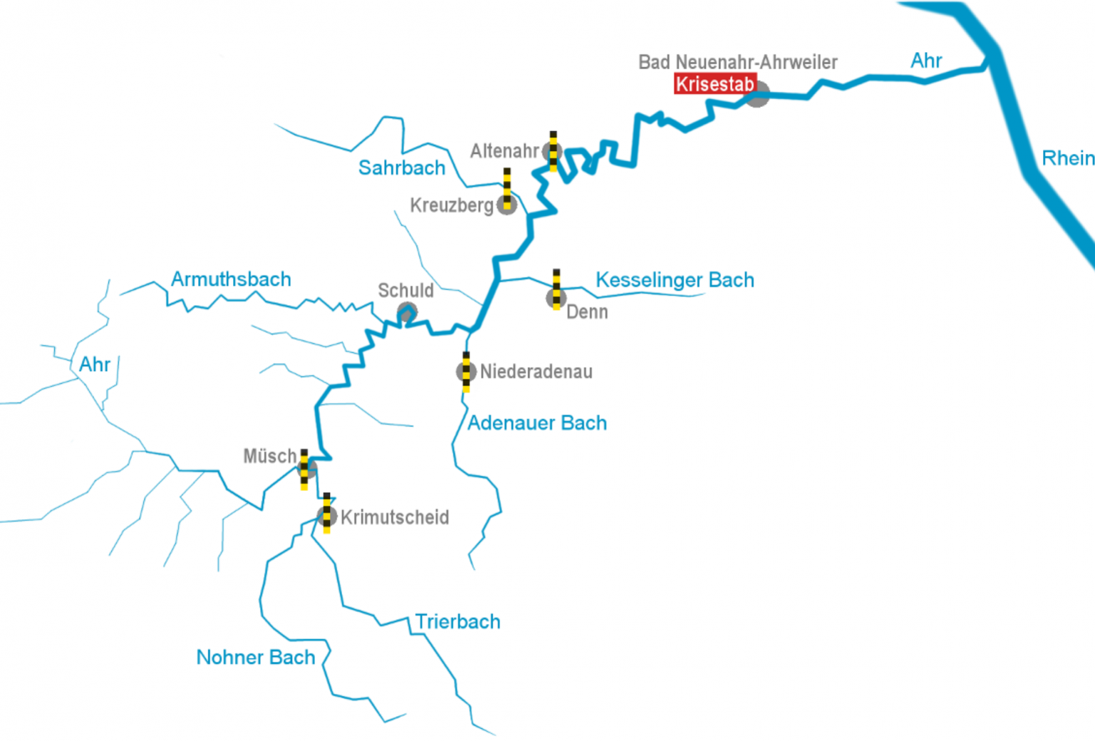
# ## Main tributaries of the Ahr
# https://wasserportal.rlp-umwelt.de/servlet/is/8181/
#
# Location | Pegelnullpunkt | Stream | Distance to Altenahr (km)
# ---: | :---: | --- | :---:
# Altenahr | 160,522 m | Ahr | 0
# Kreuzberg | 178,894 m | Sahrbach | 1.5
# Denn | 191,151 m | Kesselingerbach | 4.3
# Niederadenau | 222,015 m | Adenauerbach | 10.8
# Müsch | 292,769 m | Ahr * Trierbach | 25.5
#
# source: reitschuster.de
# Estimated average waterspeed in km/h during flooding.
# In[74]:
waterspeed= 2.5 # m/s
waterspeedkmh= waterspeed*3.6
waterspeedkmh
wiki=pd.read_html(io="https://en.wikipedia.org/wiki/Ahr", match='.+', flavor=None, header=None, index_col=None, skiprows=None, attrs=None, parse_dates=False, thousands=',', encoding=None, decimal='.', converters=None, na_values=None, keep_default_na=True, displayed_only=True)
wiki #Tributaries
# In[8]:
streams= pd.read_excel(r"Ahr.xlsx", skiprows=2,engine="openpyxl",index_col=0,na_values= "-")
streams= streams.sort_values("Elevation_Terminal", ascending=False)
streams
# In[32]:
Adenauerbach= pd.read_csv(r"Adenauerbach Aktuelle Wasserstände.csv",sep="\t", skiprows=1,usecols=[1,2],index_col=0,na_values="-")
Adenauerbach.index = pd.to_datetime(Adenauerbach.index, format="%d.%m.%Y %H:%M") # ,parse_dates=["Datum"] ,parse_dates=["Datum"]
Denn = pd.read_csv(r"Denn Aktuelle Wasserstände.csv",sep="\t", skiprows=1,usecols=[1,2],index_col=0,na_values="-")
Denn.index = pd.to_datetime(Denn.index, format="%d.%m.%Y %H:%M")
Kreuzberg =pd.read_csv(r"Kreuzberg Aktuelle Wasserstände.csv",sep="\t", skiprows=1,usecols=[1,2],index_col=0,na_values="-")
Kreuzberg.index = pd.to_datetime(Kreuzberg.index, format="%d.%m.%Y %H:%M")
Müsch= pd.read_csv(r"Müsch Aktuelle Wasserstände.csv",sep="\t", skiprows=1,usecols=[1,2],index_col=0,na_values="-")
Müsch.index = pd.to_datetime(Müsch.index, format="%d.%m.%Y %H:%M")
# In[35]:
Adenauerbach
# In[33]:
DennAbf = pd.read_csv(r"Denn Abfluss.csv",sep="\t", skiprows=1,parse_dates=["Datum"],usecols=[1,2],index_col=0,na_values="-",decimal=",",dayfirst=True)
KreuzbergAbf = pd.read_csv(r"Kreuzberg Abfluss.csv",sep="\t", skiprows=1,parse_dates=["Datum"],usecols=[1,2],index_col=0,na_values="-",decimal=",",dayfirst=True)
MüschAbf = pd.read_csv(r"Müsch Abfluss.csv",sep="\t", skiprows=1,parse_dates=["Datum"],usecols=[1,2],index_col=0,na_values="-",decimal=",",dayfirst=True)
# In[34]:
# located near Wirft, and south of Müsch
Kirmut = pd.read_csv(r"Kirmutscheid Aktuelle Wasserstände.csv",sep="\t", skiprows=1,parse_dates=["Datum"],usecols=[1,2],index_col=0,na_values="-",dayfirst=True)
KirmutAbf = pd.read_csv(r"Kirmutscheid Abfluss.csv",sep="\t", skiprows=1,parse_dates=["Datum"],usecols=[1,2],index_col=0,na_values="-",decimal=",")
# In[13]:
KirmutAbf.loc["14-07-2021 14:30": "14-07-2021 18:30"]
# In[39]:
Kirmut
# In[40]:
Kirmut["2021-07-14":"2021-07-16"].plot();
# ### Water levels of tributaries
# In[41]:
tributaries= pd.merge(Adenauerbach,Denn , left_index=True, right_index=True, suffixes=["Adenauerbach","Denn"] )
tributaries= pd.merge(tributaries ,Kreuzberg, left_index=True, right_index=True, suffixes=[None , "Kreuzberg"] )
tributaries= pd.merge(tributaries ,Müsch, left_index=True, right_index=True, suffixes=[None , "Müsch"] )
tributaries= pd.merge(tributaries ,Kirmut, left_index=True, right_index=True, suffixes=[None , "Kirmut"] )
tributaries.columns= ["Adenauerbach","Denn" ,"Kreuzberg","Müsch","Kirmut"]
# The station of Kreuzberg broke down after 18:00. That curve shows an acceleration of the water discharge by the Sahrbach.
# When we look at the rainfall values in its drainage area, we'll see that the records will be broken stream downwards.
# In[97]:
tributaries["2021-07-14":"2021-07-16"].plot( figsize=(16,5));
# ### Discharge levels of tributaries
# In[46]:
#tribut_Abf= pd.merge(Adenauerbach,Denn , left_index=True, right_index=True, suffixes=["Adenauerbach","Denn"] )
tribut_Abf= pd.merge(DennAbf ,KreuzbergAbf, left_index=True, right_index=True, suffixes=["Denn" , "Kreuzberg"] )
tribut_Abf= pd.merge(tribut_Abf ,MüschAbf, left_index=True, right_index=True, suffixes=[None , "Müsch"] )
tribut_Abf= pd.merge(tribut_Abf ,KirmutAbf, left_index=True, right_index=True, suffixes=[None , "Kirmut"] )
tribut_Abf.columns= ["Denn" ,"Kreuzberg","Müsch","Kirmut"] # "Adenauerbach",
# Adenauerbach intraday 15 minute interval data was not available, only the daily averages. Perhaps we can interpolate or make a decent regression between those 2 sets.
# In[4]:
Adenauerbach_mittelwerte_Abf= pd.read_csv(r"2718085500_Niederadenau_Messdaten_Tagesmittelwerte_Abfluss.csv",sep=",",#parse_dates=["Datum"],
index_col=2,na_values="-",decimal=".")#usecols=[1,2],
Adenauerbach_mittelwerte_Abf.index = pd.to_datetime(Adenauerbach_mittelwerte_Abf.index, format="%d.%m.%Y")
# In[5]:
Adenauerbach_mittelwerte_Abf.info()
# There have been measurements every 15 minutes, like this is the case for the other stations, for which we can calculate an outflow per day.
maybe this way gives errorsAdenauerbach_mittelwerte_Abf["Abfluss in m³/day"] = Adenauerbach_mittelwerte_Abf["Abfluss in m³/s"]*24*4
# In[6]:
Adenauerbach_mittelwerte_Abf.describe()
# In[177]:
#Adenauerbach_mittelwerte_Abf=
Adenauerbach_mittelwerte_Abf.loc["2020-07-12":"2021-07-16"]["Abfluss in m³/day"].plot(figsize=(16,5)); #.loc[:,"Abfluss in m³/s"] #
# I'm not sure that by multiplying by 24*4=96 we'll get the total discharge for the day. This can leads us to...
# In[178]:
sns.histplot( Adenauerbach_mittelwerte_Abf["Abfluss in m³/s"]);
# The histogram shows the average discharge values of the last 2 years for Adenauerbach.
# The value for 13-07-2021 is a prelude to the magnitude of the flood event the following day.
# In[ ]:
# In[ ]:
# In[ ]:
# 15 minute interval data starts at 27.06.2021 18:00, the end is 28.07.2021 23:45
# In[179]:
Adenauerbach.loc["14-07-2021 14:30": "14-07-2021 23:50"]["Wasserstand in cm"]
Adenauerbach.asfreq(freq='15M')
# In[36]:
Adenauerbach.info()
# Dropping the last hours which are nan's.
# In[181]:
Adenauerbach= Adenauerbach.dropna()
Adenauerbach.info()
# In[37]:
AdenauerbachDayMean= Adenauerbach.resample('D').mean() #["Wasserstand in cm"]on='Wasserstand in cm' Adenauerbach.resample("D").mean(); AdenauerbachDayMean["Wasserstand in cm"].tail(10)
AdenauerbachDayMean
# Perhaps it is better to bring also std into account.
# In[38]:
AdenauerbachDayStd= Adenauerbach.resample('D').std() #on='Wasserstand in cm' Adenauerbach.resample("D").mean(); AdenauerbachDayMean["Wasserstand in cm"].tail(10)
AdenauerbachDayStd
# In[57]:
AdenauerbachDayStd2= Adenauerbach["Wasserstand in cm"].rolling(3).std().fillna(method='bfill')
AdenauerbachDayStd2
# In[58]:
sns.lineplot( data=AdenauerbachDayMean);
sns.lineplot(data=AdenauerbachDayStd);
sns.lineplot(data=AdenauerbachDayStd2);
# In[70]:
sns.histplot(AdenauerbachDayMean);
# In[124]:
sns.histplot(AdenauerbachDayStd);
!pip3 install pandas==1.2.5 --user
# In[39]:
AdenauerbachDayMean.tail(35)
# #### Discharge averages for Adenauerbach
# drop values for 2021-07-28, because there are not covering the complete day.
# In[7]:
Adenauerbach_mittelwerte_Abf.info()
# In[8]:
Adenauerbach_mittelwerte_Abf.head() # Niederadenau
# In[43]:
Adenauer_mittelwerte_AbfDayMean= Adenauerbach_mittelwerte_Abf["Abfluss in m³/s"].resample('D').mean()
Adenauer_mittelwerte_AbfDayMean
Adenauer_mittelwerte_AbfDayStd= Adenauerbach_mittelwerte_Abf["Abfluss in m³/s"].resample('D', how=np.std) #on='Wasserstand in cm' Adenauerbach.resample("D").mean(); AdenauerbachDayMean["Wasserstand in cm"].tail(10)
Adenauer_mittelwerte_AbfDayStd
# In[48]:
Adenauer_mittelwerte_AbfDayStd= Adenauerbach_mittelwerte_Abf["Abfluss in m³/s"].rolling(3).std().fillna(method='bfill')
Adenauer_mittelwerte_AbfDayStd
# In[52]:
sns.lineplot ( data=Adenauer_mittelwerte_AbfDayMean.loc["July 2021"] )
sns.lineplot ( data=Adenauer_mittelwerte_AbfDayStd.loc["July 2021"] )
plt.xlim()
# In[61]:
Stdmerg= pd.merge( Adenauer_mittelwerte_AbfDayMean, Adenauer_mittelwerte_AbfDayStd, left_index=True, right_index=True, )
Stdmerg
Stdmerge= pd.merge( AdenauerbachDayMean, AdenauerbachDayStd2, left_index=True, right_index=True)
Stdmerge
# In[63]:
Stdmerger=pd.merge( Stdmerg, Stdmerge, left_index=True, right_index=True)
Stdmerger
# In[64]:
Stdmerger.plot()
# In[65]:
Stdmerger["DebitStdtoAvg"]=Stdmerger["Abfluss in m³/s_y"] / Stdmerger["Abfluss in m³/s_x"]
Stdmerger["PegelStdtoAvg"]=Stdmerger["Wasserstand in cm_y"] /Stdmerger["Wasserstand in cm_x"]
# In[66]:
Stdmerger["DebitStdtoAvg"].plot()
Stdmerger["PegelStdtoAvg"].plot()
# Select the outflow of only the complete day series for interpolation
# In[53]:
Adenauerbach_mittelwerte_AbfJuly= Adenauerbach_mittelwerte_Abf.loc["27-06-2021":"27-07-2021"][["Abfluss in m³/s"] ] # .loc
#Adenauerbach_Day_total_AbfJuly= Adenauerbach_mittelwerte_Abf.loc["27-06-2021":"27-07-2021"][["Abfluss in m³/day"] ]
Adenauerbach_mittelwerte_AbfJuly
Adenauerbach_Day_total_AbfJuly
# In[54]:
# need to be multipl with counts (nan's)
sns.scatterplot(data=AdenauerbachDayMean)
sns.scatterplot(data=Adenauerbach_mittelwerte_AbfJuly*24,color='orange') ;
# need to be multipl with counts (nan's)
sns.scatterplot(data=AdenauerbachDayMean)
sns.scatterplot(data=Adenauerbach_Day_total_AbfJuly, label="total outflow per day") ;
# In[56]:
AdenauerbachDayMean.columns
# need to be multopl with counts
# sns.scatterplot(data=AdenauerbachDayMean)
# In[190]:
sns.scatterplot(x=AdenauerbachDayMean['Wasserstand in cm'].iloc[:26], #['Wasserstand in cm'].values
y=Adenauerbach_mittelwerte_AbfJuly["Abfluss in m³/s"], #.loc["Abfluss in m³/s"].values
data=Adenauerbach_mittelwerte_AbfJuly
) ;
# In[191]:
AdenauerbachDayMean
# In[150]:
# perhaps bug in pandas
pd.__version__
# interpolating from daily to 15 minutes values.
# In[192]:
Adenauerbach_Day_total_AbfJuly.info()
# In[10]:
df=Adenauerbach_mittelwerte_AbfJuly #Adenauerbach_Day_total_AbfJuly
df = df.resample('15T').asfreq()
df
# In[11]:
df.info()
# In[12]:
Dischargeincubicmday = df.interpolate(method="cubic") # ['Abfluss in m³/day']
Dischargeincubicmday
# In[13]:
Dischargeincubicmday.plot()
df['Discharge in m³/day'] = df.interpolate(method="slinear") # ['Abfluss in m³/day']df['Discharge in m³/day'].plot()
# In[14]:
df.to_excel('Discharge.xlsx')
# divide by 96 to get back Discharge in m³/s
df['Discharge in m³/day'].loc["14-07-2021"]
# In[15]:
Dischargeincubicmday .loc["14-07-2021"]
# In[20]:
#dfD=pd.DataFrame()
Dischargeincubicm_sec= Dischargeincubicmday/96 # cos we went from 1 to 96 values # *60*15/(24*3600)
# In[21]:
Dischargeincubicm_sec.plot(); #dfD['Discharge in m³/sec']
# In[23]:
#Dischargeincubicm_sec.columns= ["Abfluss in m³/sec"]
Dischargeincubicm_sec.loc["14-07-2021"] # Abfluss in m³/day> Abfluss in m³/sec
# In[24]:
#Dischargeincubicm_sec.columns= ["Abfluss in m³/sec"]
Dischargeincubicm_sec.loc["15-07-2021"] # Abfluss in m³/day> Abfluss in m³/sec
# In[68]:
Dischargeincubicm_sec['Discharge in m³/15m']= Dischargeincubicm_sec['Abfluss in m³/s'] #ec *15*60 = overkill
Dischargeincubicm_sec['Discharge in m³/15m']
# In[70]:
Dischargeincubicm_sec['Discharge in m³/15m'].loc["14-07-2021"].sum()
# In[232]:
tribut_Abf
# In[233]:
tribut_Abf["Total"]=tribut_Abf["Denn"]+tribut_Abf["Kreuzberg"]+tribut_Abf["Müsch"]+tribut_Abf["Kirmut"]
tribut_Abfmerge= pd.merge( tribut_Abf["Total"],Dischargeincubicm_sec['Abfluss in m³/sec'], left_index=True, right_index=True,)
tribut_Abfmerge
# In[234]:
fig, ax=plt.subplots( 1,1, figsize=(16,5))
sns.lineplot( data=tribut_Abfmerge.loc["2021-07-13 12:00":"2021-07-17"]);
# In[5]:
print(14*3600, "m³/hr")
# This is not a decent method, so I'll study the rainfall-outflow balance later.
# ### The total sum of discharge of 4 principal tributaries.
# Let's compare the discharges of 4 principal tributaries with the measurements of Altenahr.
# These discharges represent 85% of the Ahr drainage area, as water levels of the Armuthsbach with 61 km² is not measured yet.
# - The (virtual) total sum is - in the beginning - 3 hours ahead of the arrival of the same discharge value in Altenahr.
# - It shortens to 2 hours when the discharges increase.
# - discharge values are derived from the water levels, and were downloaded from the RLP Umwelt site
# In[235]:
fig, ax=plt.subplots( 1,1, figsize=(16,5))
sns.lineplot( data=tribut_Abf.loc["2021-07-13 12:00":"2021-07-17"])
sns.lineplot( data=Abfluss.loc["2021-07-13 12:00":"2021-07-17"]["Abfluss in m3/s"], label="Altenahr") ;
# In[88]:
count= tribut_Abf.loc["14-07-2021 19:00":"2021-07-14 23:45"]["Müsch"].count()
recessioncoef= (tribut_Abf.loc["14-07-2021 19:00"]["Müsch"]- tribut_Abf.loc["14-07-2021 23:45"]["Müsch"])/ count
recessioncoef
# In[87]:
tribut_Abf.loc["2021-07-14 19:00"]["Müsch"]
# In[41]:
tribut_Abf["2021-07-14 18:15":"2021-07-14 23:45"]["Müsch"].count()
# Last Kreuzberg datapoint: 2718090200 14.07.2021 18:15 66,445
# Let's suppose the recession curve of the missing data is similar to that of Müsch...
def recessioncurve():
recessioncoef=3.77*np.log(66.445/320)
Q0 =66.445
curve=[]
t=24 #for t in range(1,22):
Qt= Q0* np.exp(-recessioncoef* t)
curve.append(Qt) # curve=
#Q0=Qt
return curve, Qt
recessioncurve()tribut_Abf["2021-07-14 18:30":"2021-07-16 23:45"]["Kreuzberg"]= tribut_Abf["2021-07-14 18:30":"2021-07-16 23:45"]["Müsch"]*66.445/320# merge was done, tribut_Abf["Total"]=tribut_Abf["Denn"]+tribut_Abf["Kreuzberg"]+tribut_Abf["Müsch"]+tribut_Abf["Kirmut"]
#tribut_Abfmerge['Abfluss in m³/sec']
tribut_Abfmerge['Abfluss in m³/sec'].loc["2021-07-13 12:00":"2021-07-16"].plot(figsize=(16,5));
# #### taking the time into consideration for the water flows to travel to Altenahr
# It takes some time for a flow to travel downstream from one point to another. This is done via time lags with a shift, where 1 shift equals 15 minutes later...
# In[220]:
tribut_Abfmerge["Totallags"]=tribut_Abf["Denn"].shift(2)+tribut_Abf["Kreuzberg"].shift(1)+tribut_Abf["Müsch"].shift(12)+tribut_Abf["Kirmut"].shift(14)+ tribut_Abfmerge['Abfluss in m³/sec'].shift(5)
fig,ax=plt.subplots(1,1, figsize=(16,5))
sns.lineplot( data=tribut_Abf.loc["2021-07-13 12:00":"2021-07-15 2:00"] )
sns.lineplot( data=tribut_Abfmerge.loc["2021-07-13 12:00":"2021-07-15 2:00"],marker="v", color='gold', ax=ax );
# x= dfD.loc["2021-07-13 12:00":"2021-07-15 2:00"],y= dfD['Discharge in m³/sec'].loc["2021-07-13 12:00":"2021-07-15 2:00"],
# A witness who survived the flood at Altenahr said that the peak level was about 23:00, standing at a level 30 cm higher than the level of the roof.
# In[217]:
tribut_Abfmerge.info()
sns.scatterplot( x=[222.015,191.151, 178.894, 292.769], y=tributaries.max(), data=tributaries.max()); tributaries.tail()
# In[88]:
Kirmut_WSAbf.columns
# ### Discharge - waterlevel curve for Kirmutscheid
# Trierbach waterlevel.
# In[103]:
Kirmut_WSAbf = pd.merge(Kirmut, KirmutAbf ,left_index=True, right_index=True, )
sns.scatterplot(x="Abfluss in m3/s" , y="Wasserstand in cm" , data=Kirmut_WSAbf["2021-07-14"]);
# This seems to be a theoretical derived curve, as empirical curves tend to have an increasing trend in the end, instead of a lineair.
# In[104]:
Kirmut_WSAbf.info()
# In[27]:
from scipy.integrate import trapezoid
y14pm =KirmutAbf["2021-07-14 12:00":"2021-07-14 23:45"]["Abfluss in m3/s"]
y14am =KirmutAbf["2021-07-14 00:00":"2021-07-14 11:45"]["Abfluss in m3/s"]
y147pm =KirmutAbf["2021-07-14 19:00":"2021-07-14 19:45"]["Abfluss in m3/s"]
Qpy14pm =trapezoid(y14pm, x=None, axis=- 1) #dx=15.0*60,
Qpy14am =trapezoid(y14am, x=None, axis=- 1)#dx=15.0*60,
Qpy147pm =trapezoid(y147pm, x=None, axis=- 1)# dx=45.0,
print(Qpy14am,"Abfluss in m3/12h", Qpy14pm,"Abfluss in m3/12h", Qpy147pm,"Abfluss in m3/h")
# In[21]:
100*3600
mm/hr = Flow rate (350.7 l/hr) / Area (9m^2) = 38.97mm/hr. 100mm/h total liters= 8,800,000,000
# In[25]:
0.104*3600/88000000*1000 # l/s> m³/hour / 88 km² > m² >> m/hour = 1000mm/hour
import plotly.graph_objects as go
fig = go.Figure(data=go.Cone(x=[1], y=[1], z=[1], u=[1], v=[0.5], w=[0.1]))
fig.update_layout(scene_camera_eye=dict(x=1.76, y=1.8, z=0.92))
fig.show()import plotly.graph_objects as go
fig = go.Figure(data=go.Cone(
x=[1, 2, 3],
y=[1, 2, 3],
z=[1, 2, 3],
u=[1, 0, 0],
v=[0, 3, 0],
w=[0, 0, 2],
sizemode="absolute",
sizeref=2,
anchor="tip"))
fig.update_layout(
scene=dict(domain_x=[0, 1],
camera_eye=dict(x=-0.57, y=1.36, z=0.58)))
fig.show()import plotly.graph_objects as go
fig = go.Figure(data=go.Streamtube(x=[0, 0, 0], y=[0, 1, 2], z=[0, 0, 0],
u=[0, 0, 0], v=[2, 1, 1], w=[0, 0, 0]))
fig.show()
# In[46]:
Hochwasser.columns
# ### Estimation of the volume of water/sec for a water level of 9.5 meter.
# only done to get an idea of the height of the waves
# In[26]:
from sklearn import linear_model
reg = linear_model.Lasso(alpha=0.1)
df=pd.DataFrame()
df["Wasserstand in cm"] =Ahr["2021-07-14 12:00":"2021-07-14 19:15"]["Wasserstand in cm"].to_list()
df["Abfluss in m3/s"] =Abfluss["2021-07-14 12:00":"2021-07-14 19:15"]["Abfluss in m3/s"].to_list()
pegel2volume= pd.merge(df["Wasserstand in cm"],df["Abfluss in m3/s"], left_index=True, right_index=True)
pegel2volume=pegel2volume.dropna()
#pegel2volume=pegel2volume.iloc[40:,:]
X =pegel2volume["Wasserstand in cm"].values.reshape(-1,1)
y =pegel2volume["Abfluss in m3/s"].values.reshape(-1,1)
reg.fit( X,y ,) #.values .values
reg.predict(np.array(1000).reshape(1, -1) ) # .values.reshape(1, -1)
# 1000 cm: 748.88 m³/s
# 950 cm: 707 m³/s
# 875 cm: 644.65 m³/s
# 800 cm: 582 m³/s
# In[ ]:
# In[53]:
df["Wasserstand in cm"]
# In[82]:
pegel2volume["Wasserstand in cm"].shape
# In[81]:
df["Abfluss in m3/s"].shape
# In[35]:
df["Abfluss in m3/s"].tail(20)
# ### Measurement stations of the Ahr and its tributaries.
# Messstation.xlsx
# In[42]:
Messstat= pd.read_excel("./data/Messstation.xlsx", index_col=0, engine='openpyxl',na_values="-",verbose=1,sheet_name="Blad1" ) #
Messstat=Messstat.T
Messstat["Eingerichtet"]=pd.to_datetime(Messstat["Eingerichtet"])
Messstat["Pegelnullpunkt"]=Messstat["Pegelnullpunkt"].astype(float)
Messstat["Einzugsgebiet (km2)"]=Messstat["Einzugsgebiet (km2)"].astype(float)
Messstat["Lat"]=Messstat["Lat"].astype(float)
Messstat["Long"]=Messstat["Long"].astype(float)
Messstat["Maximum_Abfluss_m³s"]=Messstat["Maximum_Abfluss_m³s"].astype(float)
Messstat["Maximum_Wasserstand"]=Messstat["Maximum_Wasserstand"].astype(float)
Messstat["HQ 100 (m³/s)"]=Messstat["HQ 100 (m³/s)"].astype(float)
Messstat["HW_waterlevel"]=Messstat["HW_waterlevel"].astype(float)
Messstat["HW_Debit"]=Messstat["HW_Debit"].astype(float)
for time in Messstat["Outage_time"]:
if time != (0 or np.nan):
Messstat["Outage_time"]=pd.to_datetime(Messstat["Outage_time"], format='%H:%M:%S') # %d/%m/%Y
else:
print(time)
pass
Messstat["Exceedance"]=Messstat["Exceedance"].astype(float)
Messstat
# In[43]:
Messstat.info()
Maximum_Abfluss_m³s Maximum_Wasserstand HQ 100 (m³/s) HW_waterlevel HW_Debit Exceedance #Outage_timeMessstatdrop.index
# ## "Highest measurements" since 1946 vs. the catastrophic flood 14-07-2021
#
# The estimation of the return intervals for "high water" were merely based on **measured, thus numerical** data. This lead to a selection of *top 10* events **since 1946**.
#
# **Historical data and writings**, letters, watermarks, were available in archives, internet and books, but were bluntly **ignored**.
#
# However, in 2014 Roggenkamp Thomas published a research with "reconstructed" estimates of outflows for the flood events of 1910 and 1804. The flood of 2016 happened, and "new record" measurements were added to the top 10 events of every station. However, Roggenkamp's work results were not added, perhaps because it does not contain return interval period estimates.
#
# Note that 2 stations were destroyed during the flood, so this plot reflects what has been measured until breaking point.
# Later on some estimations of the maxima might be added for a better insight of impact of the failure by neglecting older events.
#
# In[46]:
Messstatdrop = Messstat.drop( index='Niederadenau') # no Niederadenau
Messstatdrop.Exceedance = Messstatdrop.Exceedance*100 #(from % to real )
fig,ax= plt.subplots( 1,1,figsize=(17,5))
plt.title("Highest measurements since 1946 vs. Catastrophic flood 14-07-2021" )
sns.scatterplot(y="Maximum_Wasserstand", x="Maximum_Abfluss_m³s",data=Messstatdrop, hue="Gewässer", marker="o",size="Exceedance",palette="tab10"); #
sns.scatterplot(y="HW_waterlevel", x="HW_Debit", data=Messstatdrop, hue="Gewässer", marker="d",size="Exceedance",palette="tab10" ); # ,
plt.grid(which='both')
ax.set_xscale('log')
plt.legend (loc="lower left", bbox_to_anchor=(0.05, -0.35), ncol= 8);
#sns.barplot(x="Gewässer", y="Maximum_Wasserstand" , data=Messstat, );
# In[ ]:
df.HW_Debit.min()
# In[6]:
Messstat2= pd.read_excel("./data/Messstation.xlsx", index_col=0, engine='openpyxl',na_values="-",verbose=1,sheet_name="Blad2" ) #
Messstat2=Messstat2.T
Messstat2["Eingerichtet"]=pd.to_datetime(Messstat2["Eingerichtet"])
Messstat2["Pegelnullpunkt"]=Messstat2["Pegelnullpunkt"].astype(float)
Messstat2["Einzugsgebiet (km2)"]=Messstat2["Einzugsgebiet (km2)"].astype(float)
Messstat2["Lat"]=Messstat2["Lat"].astype(float)
Messstat2["Long"]=Messstat2["Long"].astype(float)
Messstat2["Maximum_Abfluss_m³s"]=Messstat2["Maximum_Abfluss_m³s"].astype(float)
Messstat2["Maximum_Wasserstand"]=Messstat2["Maximum_Wasserstand"].astype(float)
Messstat2["HQ 100 (m³/s)"]=Messstat2["HQ 100 (m³/s)"].astype(float)
Messstat2["HW_waterlevel"]=Messstat2["HW_waterlevel"].astype(float)
Messstat2["HW_Debit"]=Messstat2["HW_Debit"].astype(float)
for time in Messstat2["Outage_time"]:
if time != (0 or np.nan):
Messstat2["Outage_time"]=pd.to_datetime(Messstat2["Outage_time"], format='%H:%M:%S') # %d/%m/%Y
else:
print(time)
pass
Messstat2["Exceedance"]=Messstat2["Exceedance"].astype(float)
Messstat2
# With a realistic estimation of actual waterlevel
# In[7]:
Messstat2drop = Messstat2.drop( index='Niederadenau') # no Niederadenau
Messstat2drop.Exceedance = Messstat2drop.Exceedance*100 #(from % to real )
fig,ax= plt.subplots( 1,1,figsize=(17,5))
plt.title("Highest measurements since 1946 vs. Catastrophic flood 14-07-2021" )
sns.scatterplot(y="Maximum_Wasserstand", x="Maximum_Abfluss_m³s",data=Messstat2drop, hue="Gewässer", marker="o",size="Exceedance",palette="tab10"); #
sns.scatterplot(y="HW_waterlevel", x="HW_Debit", data=Messstat2drop, hue="Gewässer", marker="d",size="Exceedance",palette="tab10" ); # ,
plt.grid(which='both')
ax.set_xscale('log')
plt.legend (loc="lower left", bbox_to_anchor=(0.05, -0.35), ncol= 8);
#sns.barplot(x="Gewässer", y="Maximum_Wasserstand" , data=Messstat2, );
# ### Historical peak discharges
# These values were carefully estimated, based on good information gathered by German author Roggenkamp Thomas.
# I also added data of some noteworthy historical flood events that had casualties.
# In[31]:
peakdisch =pd.read_csv(r"Scheitelabflüsse historischer Ahr-Hochwasser.csv",parse_dates=["Date"],dayfirst=True,
sep=",",index_col=0, skipfooter=2,engine='python', na_values= "-");
peakdisch.head(10)
# we have to drop the date "30 May 1601", as pandas does not support days for dates earlier than +- 1700.
# In[33]:
peakdisch1601 = peakdisch.index[5]
peakdisch = peakdisch.drop( index="30 May 1601")
peakdisch.index = pd.to_datetime( peakdisch.index,) # euro dates\n", format='%d/%m/%Y'
#peakdisch =peakdisch.sort_index(ascending=True) # (\"Date\", inplace=True)\n",
peakdisch.head(10)
# In[5]:
print(peakdisch.iloc[0,1]/peakdisch.iloc[0,2], peakdisch.iloc[2,1]/peakdisch.iloc[2,2], peakdisch.iloc[2,0]/peakdisch.iloc[2,1])
# In[6]:
Altenahr1804= 0.9034608378870674*1208
Altenahr1804
# In[7]:
(peakdisch.iloc[0,1]/peakdisch.iloc[0,2])/ (peakdisch.iloc[2,1]/peakdisch.iloc[2,2])*( peakdisch.iloc[2,0]/peakdisch.iloc[2,1])*1208/496
# In[39]:
fig,ax=plt.subplots(2,1, figsize=(12,6.5) ,sharex=True )
sns.scatterplot(data=peakdisch.iloc[:,:4], label="discharge m³/s", ax=ax[0]);
sns.scatterplot(data=peakdisch.iloc[:,4], label="Deaths__missing_persons_excluded", ax=ax[1]); # x=peakdisch.iloc[:,4].index ,y="Deaths__missing_persons_excluded",
# In[40]:
peakdisch.iloc[:,4]
# In[41]:
peakdisch.info()
# ## Conclusions
# This is rather a place for interesting points and relevations, than a list of conclusions.
#
# - It is remarkable how many elaborate texts have been produced to establish a system for better highwater protection, alert levels and warning mechanisms etc.
# - The omission of non-measured, historical data was a capital mistake.
# - Flood event predictions were haplessly underestimated by impact and recurrence interval
# - Hence, waterlevel equipment was placed too low, and too close to the flood streams.
# - Later I found out that some station had backup sensors, which also produced inconsistent data, and failed in the end.
# - The Ahr has not been classified as a "main waterlevel river", although it has a drainage area of 900 km². This has several consequences in the field of highwater protection:
# - a highwater event does not lead to a planwise orchestrated information effort to the habitants
# - a highwater danger does not lead to a 24 hour service at the highwater notification office
# - so there was outside office hours no human supervision of the water level data of the Ahr guaranteed
# - luckily the odd data was noted by a higher level federal service, which made a correction
# ## Flood Analysis with Log-Pearson Type III Distribution
# ##### Notes:
# 1. I have based this attempt following "Streamflow Evaluations for Watershed
# Restoration Planning and Design", http://water.oregonstate.edu/streamflow/, Oregon State University, 2002-2005, which was based on the guidelines of the USGS.
# 2. The USA and USGS mainly use the Log-Pearson Type III Distribution for flood modelling, but in Europe authors seem to prefer several (General) Extreme Values models. As a consequence the variance of the regional skewness for Europe is currently under discussion. Moreover there is pretty great variation for this parameter inside the 5 Eur. regions.
#
# #### Calculator Table 1
# In[4]:
Pearson_Type_III_Calc =pd.read_excel(r"Log_Pearson_Type_III_Calculator_without2021data.xlsx",index_col=0,skipfooter=98,
usecols="J:K", skiprows=4,engine='openpyxl',); # na_values= "-"parse_dates=["Date"],
#floods["Date"] = pd.to_datetime( River_Arno.Date, format='%d/%m/%Y' ) #floods.set_index(\"Date\", inplace=True),
Pearson_Type_III_Calc.head(39)
# #### Calculator Table 2
# In[5]:
Pearson_Type_III_Calc_Tab2 =pd.read_excel(r"Log_Pearson_Type_III_Calculator_without2021data.xlsx",index_col=0,skipfooter=89,
usecols="J:P", skiprows=26,engine='openpyxl',); # na_values= "-"parse_dates=["Date"],
#floods["Date"] = pd.to_datetime( River_Arno.Date, format='%d/%m/%Y' ) #floods.set_index("Date", inplace=True),
Pearson_Type_III_Calc_Tab2.head(39)
# ### Return times in years based on only recently measured discharges.
# - The 2nd half of the table is derived from recent data, the first half is based on a timespan of 220 years of data.
# - Altenahr was chosen as focus point as it has the most historical data.
# In[39]:
AltenahrFloods =pd.read_excel(r"Ahr.xlsx",skipfooter=19, index_col=0,
usecols="A:F", skiprows=41,engine='openpyxl',sheet_name= "floods"); # na_values= "-"parse_dates=["Date"],
AltenahrFloods.style.background_gradient(axis=0, cmap='YlOrRd', low=0.05, high=1) #gmap=AltenahrFloods['Temp (c)']
#AltenahrFloods.head(9)
# In[11]:
AltenahrFloods.info()
# So based on only recent data, the model - which I doubt to be based on decent hydrological nor decent statistical knowledge - to estimate the flooded areas or the depth of the water **estimating an extreme flood**, produces a geomap on the official website pictured here:
#
# It might be the case that the data of the biggest flood of the dataset had not even been processed in the model.
#
# The map for a less worse *"100 year flood"* is added under for comparison.
#
#
# In case you see a clear difference in less than 15 seconds, you must have the eyesight of an eagle.
# In[ ]:
# ### Return times in years based on 220 years of realistic discharge data.
# Altenahr was chosen as focus point as it has the most historical data.
# In[14]:
fig, ax = plt.subplots(1, 1, figsize=(14,6))
sns.lineplot(x="Tr for Altenahr ", y="Q Tr m³/s" , data=AltenahrFloods,marker="o",label="Data starts 1804" ); #log_x=True,
sns.lineplot(x="Jährlichkeiten Abfluss in m3/s", y="Abfluss [m³/s]", data=AltenahrFloods,marker="o",label="Data starts 1946",color="r",markerfacecolor="crimson" ); #log_x=True,
plt.grid(b=True, which='minor', axis='both')
plt.xscale("log")
# Roggenkamp T. estimated the recent flood had a discharge of about 800 m³/s. I think this number will get a bit higher when the waterlevels or outflows of the Adenauerbach station, if ever, get published.
# According to this plot we have a return period of 40 years for that discharge value.
# Let's hope more useful data gets retrieved...
# peak level of the flood: see the bar tagged on the chimney
#
# In[16]:
fig, ax = plt.subplots(1, 1, figsize=(14,6)); sns.regplot(x=AltenahrFloods.index, y="LogQ Tr m³s", data=AltenahrFloods,logx=True,ci=95 ); #"Tr for Altenahr "
plt.grid(b=True, which='minor', axis='both'); plt.ylim(2,3.4)
plt.xscale("log")
sns.regplot?sns.lineplot?
# In[18]:
fig, ax = plt.subplots(1, 1, figsize=(14,6)); sns.regplot(x=AltenahrFloods.index, y="Q Tr m³/s" , data=AltenahrFloods,logx=True,ci=95); #"Tr for Altenahr "
plt.grid(b=True, which='minor', axis='both'); plt.ylim(0,1300)
plt.xscale("log")
# In[ ]:
# ## Fit several distributions
# module reliability
# ### Water levels of 1st flood day
# In[77]:
from reliability.Distributions import Exponential_Distribution
from reliability.Probability_plotting import Exponential_probability_plot
import matplotlib.pyplot as plt
from reliability.Other_functions import make_right_censored_data
#dist = Exponential_Distribution(Lambda=0.25, gamma=12)
raw_data =Ahr["2021-07-14 12:00":"2021-07-14 19:45"]["Wasserstand in cm"].values # dist.random_samples(100, seed=42)draw some random data from an exponential distribution
#data = make_right_censored_data(raw_data, threshold=17) # right censor the data at 17
Exponential_Distribution(Lambda=0.75).CDF(linestyle='--', label='True CDF') # we can't plot dist because it will be location shifted
Exponential_probability_plot(failures=raw_data, fit_gamma=False) # do the probability plot. Note that we have specified to fit gamma
plt.legend()
plt.show()
# In[31]:
1/0.00444
# As the hydrostation got destroyed, it might be ok to improvise some missing levels and fit again.
# In[29]:
from reliability.Fitters import Fit_Everything
data = Ahr["2021-07-14 12:00":"2021-07-14 22:45"]["Wasserstand in cm"].dropna() # created using Weibull_Distribution(alpha=5,beta=2), and rounded to nearest int
data =data.values
Fit_Everything(failures=data, show_histogram_plot=True, show_probability_plot=True, show_PP_plot=True, show_best_distribution_probability_plot=True)
# In[30]:
from reliability.Fitters import Fit_Everything
data = Hochwasser["Wasserstand in cm"].values # created using Weibull_Distribution(alpha=5,beta=2), and rounded to nearest int
Fit_Everything(failures=data, show_histogram_plot=True, show_probability_plot=True, show_PP_plot=True, show_best_distribution_probability_plot=True)
# In[ ]:
# In[57]:
from scipy.stats import gumbel_r
import matplotlib.pyplot as plt
fig, ax = plt.subplots(1, 1)
#Calculate the first four moments: mean, var, skew, kurt = gumbel_r.stats(moments='mvsk')
#Display the probability density function (pdf): x = np.linspace(gumbel_r.ppf(0.01), gumbel_r.ppf(0.99), 100)
x=[100,200,300,350,375,400,425,450,500,550,600,650,700,800,900]
ax.plot(x, gumbel_r.pdf(x, loc=444.438, scale=65.035), 'r-', lw=1, alpha=0.6, label='gumbel_r pdf');
# In[64]:
gumbel_r.pdf(700, loc=444.438, scale=65.035)
# In[58]:
gumbel_r.pdf(900, loc=444.438, scale=65.035)
# In[63]:
1/215*gumbel_r.pdf(900, loc=444.438, scale=65.035) # 365.25*
# ### yearly maxima
# In[96]:
from reliability.Fitters import Fit_Everything
raw_data =klima_jahr_1930.JA_MX_RS.dropna() # dist.random_samples(100, seed=42)draw some random data from an exponential distributio
raw_data =raw_data.values
new_arr = np.delete(raw_data, [1])
#data = Hochwasser["Wasserstand in cm"].values # created using Weibull_Distribution(alpha=5,beta=2), and rounded to nearest int
Fit_Everything(failures=new_arr, show_histogram_plot=True, show_probability_plot=True, show_PP_plot=True, show_best_distribution_probability_plot=True)
This parametrization corresponds to setting 's'= sigma and 'scale'= exp(mu).
# In[97]:
np.exp(3.51167)
# In[98]:
from scipy.stats import lognorm
import matplotlib.pyplot as plt
fig, ax = plt.subplots(1, 1)
raw_data =klima_jahr_1930.JA_MX_RS.dropna() # dist.random_samples(100, seed=42)draw some random data from an exponential distributio
x = raw_data.values # np.linspace(lognorm.ppf(0.01, s), lognorm.ppf(0.99, s), 100)
ax.plot(x, lognorm.pdf(x, s=33.5, loc=3.51167, scale= 0.284678), #
'r+', lw=1.5, alpha=0.6, label='lognorm pdf');
# that minimum is an outlier, and should be deleted
# In[91]:
type(raw_data.values)
new_arr = np.delete(raw_data.values, [1])
# In[101]:
from scipy.stats import lognorm
import matplotlib.pyplot as plt
fig, ax = plt.subplots(1, 1)
#raw_data =klima_jahr_1930.JA_MX_RS.dropna() # dist.random_samples(100, seed=42)draw some random data from an exponential distributio
x = new_arr # np.linspace(lognorm.ppf(0.01, s), lognorm.ppf(0.99, s), 100)
ax.plot(x, lognorm.pdf(x, s=33.227, loc=3.51167, scale= 0.284678), #
'r+', lw=1.5, alpha=0.6, label='lognorm pdf');
# In[100]:
lognorm.pdf(100, s=33.5, loc=3.51167, scale= 0.284678)
# In[99]:
1/lognorm.pdf(100, s=33.5, loc=3.51167, scale= 0.284678)
# In[83]:
from scipy.stats import lognorm
def test_fix_fit_2args_lognorm(self):
"""Regression test for #1551."""
np.random.seed(12345)
with np.errstate(all='ignore'):
x = lognorm.rvs(0.25, 0., 20.0, size=20)
np.allclose(np.array( lognorm.fit(x, loc=0, scale=20)), # assert
[0.25888672, 0, 20], atol=1e-5)
test_fix_fit_2args_lognorm(20)
lognorm.pdf??
# In[ ]:
 #
#  # ## High water level events of the Ahr
# It is actually easy to find many sources with good information online: *google "hochwasser der Ahr"*
# - Beim Hochwasser am 21. Juli 1804 starben 64 Menschen. Beim Hochwasser am 13. Juni 1910 starben 57 *(or 150?)* Menschen;[9] danach mussten alle Ahr-Brücken – außer der bei Rech – wiederaufgebaut werden. Im Ahrstraßentunnel in Altenahr sind Marken der höchsten Pegel angebracht.
#
# - Am 2. Juni 2016 erreichte der Pegel der Ahr in Kreuzberg und Altenahr seinen seit Messbeginn bis dahin höchsten Stand. Am Pegel Altenahr stieg die Ahr auf 369 Zentimeter, 20 cm mehr als beim zuvor höchsten Hochwasser 1993.[10]
#
# - Im Laufe des 14. Juli 2021 führten starke und anhaltende Regenfälle zu den bisher höchsten Pegelständen, die jemals gemessen wurden. Die Messstation in Altenahr gab um 20:45 Uhr einen Pegelstand von 575 cm an[11] und in Bad Bodendorf am 15. Juli 2021 um 03:45 Uhr einen Stand von 483 cm.[12] Am 14. Juli 2021 erreichte der Pegel Altenahr einen Wasserstand von etwa 700 cm.[13] Somit wurden die Pegelstände des „Jahrhunderthochwassers“[14] von 2016 um rund 3,3 Meter übertroffen.
#
# - Heimatforscher Dr. Hans Frick, der das Hochwasser von 1804 im Jahre 1929 als Erster umfassend darstellte: Jede Vorsorge war nutzlos, denn so hoch hatte die Ahr bis dahin noch nie gestanden. Über der Steinbrücke bei Rech soll sie eine Höhe von acht Fuß (etwa 2,50 Meter) erreicht haben... Fast alle Ahrbrücken – einer Aufstellung nach 30 Stück – stürzten ein, auch die aus Stein. Nach der gleichen Quelle verschwand auch der 18 Fuß (5,50 Meter) über normalem Wasserstand der Ahr gelegene Stotzheimer Hof bei Rech spurlos.
#
# Dr. Hans Frick was the first geographer who searched for historical source materials which dated more than 100 years ago.
# Here are translations of some of the old texts, and citation from Hr. Seel: „Die Ahr und ihre Hochwässer in alten Quellen“ :
#
# - On May 30th 1601, “what day has been the Lord's Ascension evening”, the sky darkened in the afternoon, according to the chronicle from the village of Antweiler. A "thunderstorm" with rain and hail "fell down" so forceful that the residents believed in the end of the world. The subsequent flood "suffered other great damage with 16 buildings, houses, sheds and places and 9 people drowned." In a village in which only about 180 souls lived at that time.
#
# - The Antweiler Chronicle **does not report how great the damage was further downstream** in Anno Domini 1601. But one can assume that they were also considerable, because Antweiler is located on the upper reaches of the Ahr and the tidal wave of the "storm" flowed further downstream, then as now. About ten kilometers away in the village of Schuld, which was hit particularly hard by the floods last week. *The similarity with the build up and the damage of the 2021 flood is striking.*
#
# - Tuesday, August 1, 1719. This time too, the Ahr emerged from its river bed. Not as devastating as 118 years ago but with power. The chronicle of the monastery on Kalvarienberg in today's Bad Neuenahr-Ahrweiler reports that a wall in Heppingen was simply "overturned" by the flood, as was an avenue whose posts were "driven as far as Lorsdorf", i.e. about two current kilometers by car downstream. Two servants and an administrator of the monastery had only been able to save themselves in the trees until "help" came. The water had come so quickly.
# - The flood had also caused damage to the upper reaches of the Ahr, for example the village chapel in Schuld, which had only been built 20 years earlier, had to be completely renovated.
#
#
# - July 21, 1804: According to reports from the French authorities responsible at the time, the Ahr had been flooding for days when a storm followed on July 21. Within a short time all tributaries swelled up. Then the tide came. In today's Bad Neuenahr-Ahrweiler a chronicler wrote that the whole "getraidt was flooded". And Pastor Fey in Bodendorf, six kilometers downriver, noted in his diary: 'On July 21st, I went with Herr[n] Dean Radermacher over the mountain to Remagen [on the Rhine] and it started to rain this hard on top of the mountain so that we both arrived in Remagen soaked to the skin. In the same night the Ahr grew so much that ... all possible household utensils, timber and dead people were found in the field who had been driven there with the Ahr.'
#
# - Fields washed away down to the rock.
#
# - A plaque in the community center of Dorsel on the upper reaches of the Ahr still reminds of the devastating flood of 1804: “21. Julius at 3 o'clock in the afternoon, during a terrible thunderstorm coming from the north, the water fell in streams from the clouds, causing the bottom to flow from many fields to the rocks ... [and] the steel foundry suddenly "wiped out". The water covered "large masses of earth, sand, hedges and shrubs" and also tore away the "very strong stone foundry bridge".
#
# - The only reminder of the Dorsel steel foundry, to which the bridge belonged, is the campsite of the same name.
#
# - A total of 63 people were killed in the disaster. The same happened to many horses, draft cattle and feeder cattle. A total of 129 houses, 162 barns and stables, 18 mills, eight blacksmiths and almost all bridges were destroyed. Another 469 houses, 234 barns and stables, two mills and a forge were damaged. Churches and houses were almost without exception under water. Fruit trees were uprooted, vineyards washed away, the harvest destroyed and the meadows of the floodplains silted up with gravel and rubble.
#
# ### The top 10 high water events 1946 - 2019
# ... to which I added the estimated, sts. calculated, values of some historical flood events.
# In[43]:
Hochwasser= Hochwasser.sort_index( ascending=True)
Hochwasser.head(19)
a provisional estimation of the drainage area:if Hochwasser.iloc[:,2]!= np.nan :
Hochwasser["km2"]= Hochwasser.iloc[:,1]/Hochwasser.iloc[:,2]*1000
elif Hochwasser.iloc[:,2]!= "" :
Hochwasser["km2"]= Hochwasser.iloc[:,1]/Hochwasser.iloc[:,2]*1000
else:
Hochwasser["km2"]= np.nanHochwasser2= Hochwasser.iloc[:,2].astype('Int64')
Hochwasser1 =Hochwasser.iloc[:,1].astype('Int64') #Hochwasser1 /
Hochwasserlist =[Hochwasser1/int(x)*1000 for x in Hochwasser2 if x != np.nan if x != "" ]
Hochwasserlist
# ["km2"]else np.nan
# elif Hochwasser.iloc[:,2]!= "" : Hochwasser["km2"]= Hochwasser.iloc[:,1]/Hochwasser.iloc[:,2]*1000
#else: Hochwasser["km2"]=type(Hochwasserlist)type(Hochwasserlist[0])Hochwasser["km2"]=Hochwasserlist[0]
# Hochwasser2021= Hochwasser[~Hochwasser.iloc[6,:] ] #Hochwasser= "1993-12-01"
# Hochwasser2021
# In[45]:
Hochwasser.iloc[6,:]
# In[46]:
Hochwasser.info()
# In[47]:
Hochwasser[Hochwasser["Nr."]==14]
# - the former lowest value in the official list of top 10 HW events should go as I inserted the 2021 event
# - calculate the time interval between the events of flooding > recurrence interval
# In[48]:
Hochwasser["year"]= Hochwasser.index.year
Hochwasser["years"]=2021.5- Hochwasser["year"] # avoid 0
import datetime
today = datetime.date.today()
Hochwasser["days"]= (pd.to_datetime(today) - Hochwasser.index).days
import datetime
today = datetime.date.today()
dt= pd.to_datetime('1910/06/13', format='%Y/%m/%d') # date of earlier big flood 1946/08/01
Timesbetween= []
for ind in Hochwasser.index:
dt1= ind
print( dt1)
interval= (dt1-dt).days
print( interval)
#Timesbetween= Timesbetween+ list(interval)
dt =dt1
print( pd.to_datetime(today), (pd.to_datetime(today) -ind).days)
#Timesbetween
# In[246]:
pd.to_datetime('1910/06/13', format='%Y/%m/%d')-pd.to_datetime('2021/07/26', format='%Y/%m/%d')
intervals={"1910-06-13 00:00:00":40586,
"1961-01-31 00:00:00":5297,
"1966-11-12 00:00:00":2111,
"1984-05-30 00:00:00":6409,
"1984-07-02 00:00:00":33,
"1984-11-23 00:00:00":144,
"1988-03-16 00:00:00":1209,
"1993-12-21 00:00:00":2106, # the former lowest val should go as I inserted the 2021 event
"1995-01-23 00:00:00":398,
#"1993-12-21 00:00:00":20,
"2016-02-06 00:00:00":7684,
"2021-07-14 00:00:00":1985}
intervals= pd.DataFrame.from_dict(intervals, orient='index',columns=['TimeInterval']) #index= intervals[0]
type(intervals)intervals.plot();intervals.info()int10= intervals.index
int10
# In[50]:
fig,ax=plt.subplots( 1,1, figsize=(12,5))
sns.scatterplot(x=Hochwasser["Abfluss in m3/s"] ,y=Hochwasser.years, data=Hochwasser,hue=Hochwasser["year"],palette="magma")#hue=int10 [:-1]
plt.xscale("log") #ax.xaxis_scale("log")
# In[51]:
fig,ax=plt.subplots( 1,1, figsize=(12,6))
sns.scatterplot(x=Hochwasser["years"] ,y=Hochwasser["Wasserstand in cm"].values, data=Hochwasser,hue=Hochwasser["year"],palette="magma")#hue=int10
plt.xscale("log") #ax.xaxis_scale("log")
plt.legend() ;
#
# ## High water level events of the Ahr
# It is actually easy to find many sources with good information online: *google "hochwasser der Ahr"*
# - Beim Hochwasser am 21. Juli 1804 starben 64 Menschen. Beim Hochwasser am 13. Juni 1910 starben 57 *(or 150?)* Menschen;[9] danach mussten alle Ahr-Brücken – außer der bei Rech – wiederaufgebaut werden. Im Ahrstraßentunnel in Altenahr sind Marken der höchsten Pegel angebracht.
#
# - Am 2. Juni 2016 erreichte der Pegel der Ahr in Kreuzberg und Altenahr seinen seit Messbeginn bis dahin höchsten Stand. Am Pegel Altenahr stieg die Ahr auf 369 Zentimeter, 20 cm mehr als beim zuvor höchsten Hochwasser 1993.[10]
#
# - Im Laufe des 14. Juli 2021 führten starke und anhaltende Regenfälle zu den bisher höchsten Pegelständen, die jemals gemessen wurden. Die Messstation in Altenahr gab um 20:45 Uhr einen Pegelstand von 575 cm an[11] und in Bad Bodendorf am 15. Juli 2021 um 03:45 Uhr einen Stand von 483 cm.[12] Am 14. Juli 2021 erreichte der Pegel Altenahr einen Wasserstand von etwa 700 cm.[13] Somit wurden die Pegelstände des „Jahrhunderthochwassers“[14] von 2016 um rund 3,3 Meter übertroffen.
#
# - Heimatforscher Dr. Hans Frick, der das Hochwasser von 1804 im Jahre 1929 als Erster umfassend darstellte: Jede Vorsorge war nutzlos, denn so hoch hatte die Ahr bis dahin noch nie gestanden. Über der Steinbrücke bei Rech soll sie eine Höhe von acht Fuß (etwa 2,50 Meter) erreicht haben... Fast alle Ahrbrücken – einer Aufstellung nach 30 Stück – stürzten ein, auch die aus Stein. Nach der gleichen Quelle verschwand auch der 18 Fuß (5,50 Meter) über normalem Wasserstand der Ahr gelegene Stotzheimer Hof bei Rech spurlos.
#
# Dr. Hans Frick was the first geographer who searched for historical source materials which dated more than 100 years ago.
# Here are translations of some of the old texts, and citation from Hr. Seel: „Die Ahr und ihre Hochwässer in alten Quellen“ :
#
# - On May 30th 1601, “what day has been the Lord's Ascension evening”, the sky darkened in the afternoon, according to the chronicle from the village of Antweiler. A "thunderstorm" with rain and hail "fell down" so forceful that the residents believed in the end of the world. The subsequent flood "suffered other great damage with 16 buildings, houses, sheds and places and 9 people drowned." In a village in which only about 180 souls lived at that time.
#
# - The Antweiler Chronicle **does not report how great the damage was further downstream** in Anno Domini 1601. But one can assume that they were also considerable, because Antweiler is located on the upper reaches of the Ahr and the tidal wave of the "storm" flowed further downstream, then as now. About ten kilometers away in the village of Schuld, which was hit particularly hard by the floods last week. *The similarity with the build up and the damage of the 2021 flood is striking.*
#
# - Tuesday, August 1, 1719. This time too, the Ahr emerged from its river bed. Not as devastating as 118 years ago but with power. The chronicle of the monastery on Kalvarienberg in today's Bad Neuenahr-Ahrweiler reports that a wall in Heppingen was simply "overturned" by the flood, as was an avenue whose posts were "driven as far as Lorsdorf", i.e. about two current kilometers by car downstream. Two servants and an administrator of the monastery had only been able to save themselves in the trees until "help" came. The water had come so quickly.
# - The flood had also caused damage to the upper reaches of the Ahr, for example the village chapel in Schuld, which had only been built 20 years earlier, had to be completely renovated.
#
#
# - July 21, 1804: According to reports from the French authorities responsible at the time, the Ahr had been flooding for days when a storm followed on July 21. Within a short time all tributaries swelled up. Then the tide came. In today's Bad Neuenahr-Ahrweiler a chronicler wrote that the whole "getraidt was flooded". And Pastor Fey in Bodendorf, six kilometers downriver, noted in his diary: 'On July 21st, I went with Herr[n] Dean Radermacher over the mountain to Remagen [on the Rhine] and it started to rain this hard on top of the mountain so that we both arrived in Remagen soaked to the skin. In the same night the Ahr grew so much that ... all possible household utensils, timber and dead people were found in the field who had been driven there with the Ahr.'
#
# - Fields washed away down to the rock.
#
# - A plaque in the community center of Dorsel on the upper reaches of the Ahr still reminds of the devastating flood of 1804: “21. Julius at 3 o'clock in the afternoon, during a terrible thunderstorm coming from the north, the water fell in streams from the clouds, causing the bottom to flow from many fields to the rocks ... [and] the steel foundry suddenly "wiped out". The water covered "large masses of earth, sand, hedges and shrubs" and also tore away the "very strong stone foundry bridge".
#
# - The only reminder of the Dorsel steel foundry, to which the bridge belonged, is the campsite of the same name.
#
# - A total of 63 people were killed in the disaster. The same happened to many horses, draft cattle and feeder cattle. A total of 129 houses, 162 barns and stables, 18 mills, eight blacksmiths and almost all bridges were destroyed. Another 469 houses, 234 barns and stables, two mills and a forge were damaged. Churches and houses were almost without exception under water. Fruit trees were uprooted, vineyards washed away, the harvest destroyed and the meadows of the floodplains silted up with gravel and rubble.
#
# ### The top 10 high water events 1946 - 2019
# ... to which I added the estimated, sts. calculated, values of some historical flood events.
# In[43]:
Hochwasser= Hochwasser.sort_index( ascending=True)
Hochwasser.head(19)
a provisional estimation of the drainage area:if Hochwasser.iloc[:,2]!= np.nan :
Hochwasser["km2"]= Hochwasser.iloc[:,1]/Hochwasser.iloc[:,2]*1000
elif Hochwasser.iloc[:,2]!= "" :
Hochwasser["km2"]= Hochwasser.iloc[:,1]/Hochwasser.iloc[:,2]*1000
else:
Hochwasser["km2"]= np.nanHochwasser2= Hochwasser.iloc[:,2].astype('Int64')
Hochwasser1 =Hochwasser.iloc[:,1].astype('Int64') #Hochwasser1 /
Hochwasserlist =[Hochwasser1/int(x)*1000 for x in Hochwasser2 if x != np.nan if x != "" ]
Hochwasserlist
# ["km2"]else np.nan
# elif Hochwasser.iloc[:,2]!= "" : Hochwasser["km2"]= Hochwasser.iloc[:,1]/Hochwasser.iloc[:,2]*1000
#else: Hochwasser["km2"]=type(Hochwasserlist)type(Hochwasserlist[0])Hochwasser["km2"]=Hochwasserlist[0]
# Hochwasser2021= Hochwasser[~Hochwasser.iloc[6,:] ] #Hochwasser= "1993-12-01"
# Hochwasser2021
# In[45]:
Hochwasser.iloc[6,:]
# In[46]:
Hochwasser.info()
# In[47]:
Hochwasser[Hochwasser["Nr."]==14]
# - the former lowest value in the official list of top 10 HW events should go as I inserted the 2021 event
# - calculate the time interval between the events of flooding > recurrence interval
# In[48]:
Hochwasser["year"]= Hochwasser.index.year
Hochwasser["years"]=2021.5- Hochwasser["year"] # avoid 0
import datetime
today = datetime.date.today()
Hochwasser["days"]= (pd.to_datetime(today) - Hochwasser.index).days
import datetime
today = datetime.date.today()
dt= pd.to_datetime('1910/06/13', format='%Y/%m/%d') # date of earlier big flood 1946/08/01
Timesbetween= []
for ind in Hochwasser.index:
dt1= ind
print( dt1)
interval= (dt1-dt).days
print( interval)
#Timesbetween= Timesbetween+ list(interval)
dt =dt1
print( pd.to_datetime(today), (pd.to_datetime(today) -ind).days)
#Timesbetween
# In[246]:
pd.to_datetime('1910/06/13', format='%Y/%m/%d')-pd.to_datetime('2021/07/26', format='%Y/%m/%d')
intervals={"1910-06-13 00:00:00":40586,
"1961-01-31 00:00:00":5297,
"1966-11-12 00:00:00":2111,
"1984-05-30 00:00:00":6409,
"1984-07-02 00:00:00":33,
"1984-11-23 00:00:00":144,
"1988-03-16 00:00:00":1209,
"1993-12-21 00:00:00":2106, # the former lowest val should go as I inserted the 2021 event
"1995-01-23 00:00:00":398,
#"1993-12-21 00:00:00":20,
"2016-02-06 00:00:00":7684,
"2021-07-14 00:00:00":1985}
intervals= pd.DataFrame.from_dict(intervals, orient='index',columns=['TimeInterval']) #index= intervals[0]
type(intervals)intervals.plot();intervals.info()int10= intervals.index
int10
# In[50]:
fig,ax=plt.subplots( 1,1, figsize=(12,5))
sns.scatterplot(x=Hochwasser["Abfluss in m3/s"] ,y=Hochwasser.years, data=Hochwasser,hue=Hochwasser["year"],palette="magma")#hue=int10 [:-1]
plt.xscale("log") #ax.xaxis_scale("log")
# In[51]:
fig,ax=plt.subplots( 1,1, figsize=(12,6))
sns.scatterplot(x=Hochwasser["years"] ,y=Hochwasser["Wasserstand in cm"].values, data=Hochwasser,hue=Hochwasser["year"],palette="magma")#hue=int10
plt.xscale("log") #ax.xaxis_scale("log")
plt.legend() ;
#  #
# 
 # This Image by Roggenkamp T. and co. Herget lays bare the drama of the fall out of the hydrometers. I guess the peak in Altenahr arrived at or just after midnight. These authors say that the tributary Sahrbach had a big impact on the pegel in Altenahr, so I take a look at the public available measure station there: Kreuzberg. [source: ](https://www.faz.net/aktuell/wissen/erde-klima/flutkatastrophe-im-ahrtal-neue-erkenntnisse-zum-hochwasser-17470847.html)
# ### Estimated parameters of the 1910 flood in Bad Neuenahr
# In[59]:
flood1910= pd.read_excel(r"Ahr2.xlsx", skiprows=1,engine="openpyxl",index_col=0,na_values= "", sheet_name="flood_1910")
flood1910T= flood1910.iloc[:,:4].T
flood1910T
# In[63]:
sns.scatterplot( data=flood1910T ,)
plt.yscale("log")
# ## Main tributaries of the Ahr
# https://wasserportal.rlp-umwelt.de/servlet/is/8181/
#
# Location | Pegelnullpunkt | Stream | Distance to Altenahr (km)
# ---: | :---: | --- | :---:
# Altenahr | 160,522 m | Ahr | 0
# Kreuzberg | 178,894 m | Sahrbach | 1.5
# Denn | 191,151 m | Kesselingerbach | 4.3
# Niederadenau | 222,015 m | Adenauerbach | 10.8
# Müsch | 292,769 m | Ahr * Trierbach | 25.5
#
#
# This Image by Roggenkamp T. and co. Herget lays bare the drama of the fall out of the hydrometers. I guess the peak in Altenahr arrived at or just after midnight. These authors say that the tributary Sahrbach had a big impact on the pegel in Altenahr, so I take a look at the public available measure station there: Kreuzberg. [source: ](https://www.faz.net/aktuell/wissen/erde-klima/flutkatastrophe-im-ahrtal-neue-erkenntnisse-zum-hochwasser-17470847.html)
# ### Estimated parameters of the 1910 flood in Bad Neuenahr
# In[59]:
flood1910= pd.read_excel(r"Ahr2.xlsx", skiprows=1,engine="openpyxl",index_col=0,na_values= "", sheet_name="flood_1910")
flood1910T= flood1910.iloc[:,:4].T
flood1910T
# In[63]:
sns.scatterplot( data=flood1910T ,)
plt.yscale("log")
# ## Main tributaries of the Ahr
# https://wasserportal.rlp-umwelt.de/servlet/is/8181/
#
# Location | Pegelnullpunkt | Stream | Distance to Altenahr (km)
# ---: | :---: | --- | :---:
# Altenahr | 160,522 m | Ahr | 0
# Kreuzberg | 178,894 m | Sahrbach | 1.5
# Denn | 191,151 m | Kesselingerbach | 4.3
# Niederadenau | 222,015 m | Adenauerbach | 10.8
# Müsch | 292,769 m | Ahr * Trierbach | 25.5
#
#