 #
#  #
#
#
#  #
#  #
# In[9]:
mome=list("ABCDEF")
genes=[list("ABCD"),list("CDEF")]
g=set(genes[1])
i=2
proc=lambda g,h:"".join(list(g.difference(g.intersection(set(h)))))
[proc(g,m) for m in mome]
# In[31]:
qplan=np.array([[(i>>(j))%2>0 for j in range(3)] for i in range(8)])
pA,pB,pC=qplan.T
fplan=np.array([pA,pB,pC,pA*pB*pC]).T#np.array(list(qplan.T)+[qplan[:,0]*qplan[:,1],qplan[:,2]*qplan[:,1]]).T
zome=np.array(mome[:4])
["".join(zome[q]) for q in fplan]
# Example
# =============
# ### mapping reflectivity on grown oxide
# In[147]:
pl.plot(bix,dd[2:,10])
pl.plot(bix,dd[2:,60])
pl.xlim(2.6,4)
pl.xlabel("energy [eV]")
pl.ylabel("relat. reflectivity")
pl.axvspan(3.0,3.2,alpha=0.3)
pl.axvspan(3.4,3.6,alpha=0.3,color='y')
pl.grid()
pl.ylim(0,1.5);
pl.savefig("waf_spec_example.png")
# - not attempting to model spectral response - only **average reflectivity** of a selected narrow band (virtual filter)
# In[ ]:
#bix=sm.bands[10].ix
px1,py1=dd[0,1:],dd[1,1:]
bix=dd[2:,0]
zsel1=abs(bix-3.5)<0.1
#vs1=np.array([b.iy[zsel1].mean() for b in sm.bands])
vs1=dd[2:,1:][zsel1].mean(0)
zsel2=abs(bix-3.1)<0.1
#vs2=np.array([b.iy[zsel2].mean() for b in sm.bands])
vs2=dd[2:,1:][zsel2].mean(0)
chsel=(vs1>0.8)*(vs1<1)
px1=px1[chsel]
py1=py1[chsel]
vs2=vs2[chsel]
vs1=vs1[chsel]
# we select upper band (stronger signal)
# In[122]:
pl.plot(px1,vs2,'+',label="band 3.1eV")
pl.plot(px1,vs1,'+',label="band 3.5eV")
pl.xlabel("x distance")
pl.ylabel("relat. reflectivity")
pl.legend()
#pl.ylim(0.8,1)
pl.savefig("waf_orig_disp.png")
vs.min(),vs.max()
# y-dependence seems to follow a sinusoidal wave
# In[128]:
pl.plot(py1,vs,'+')
pl.ylabel("relat. reflectivity")
pl.xlabel("y distance")
pl.savefig("waf_disp_y.png");
#pl.ylim(0.8,1)
# In[125]:
frac=lambda q:q-int(q)
def gdif(yper=70,rep=0):
mat=np.array([np.cos(2*np.pi*py1/yper),np.sin(2*np.pi*py1/yper),np.ones_like(py1)]).T
hess=mat.T.dot(mat)
pars=np.linalg.inv(hess).dot(mat.T).dot(vs)
if rep==1: return pars
if rep==2: return mat.dot(pars)
return vs-mat.dot(pars)
pl.plot(py1,gdif(72),'+')
pl.ylabel("relat. reflectivity")
pl.xlabel("y distance")
pl.title("sinusoid. model subtracted")
pl.savefig("waf_disp_y_sub72.png");
# testing a range of periods
# - linear model in amplitude + phase + offset ($p_0 + p_1\ \cos y/d + p_2\ \sin y/d$)
# - non-linear optimization in 1 variable only
# In[129]:
lper=np.r_[60:110]
pl.plot(lper,[(gdif(l)**2).sum() for l in lper])
from scipy import optimize as op
pst=op.fmin(lambda p:(gdif(p)**2).sum(),[75])[0]
pl.ylabel("sum of resid.^2")
pl.xlabel("period [mm]")
pl.savefig("waf_period_min.png");
pst,gdif(pst,1)
# subtracting model for y-axis variance was reduced to 40%
#
# - now back to x-dependence
# In[135]:
psuby=gdif(pst)
pl.plot(px1,psuby,'+')
pl.xlabel("x position")
pl.ylabel("y-depend. subtracted");
pl.savefig("waf_disp_x.png");
from scipy import ndimage as nd
ovar=nd.variance(vs,px1,np.unique(px1))
nvar=nd.variance(psuby,px1,np.unique(px1))
print("reducing by subtracting y depend.")
ovar.sum(),nvar.sum()
# another reduction by 35% by subtracting 3-rd order polynomial
# In[137]:
xfit=np.polyfit(px1,psuby,3)
xlin,ylin=np.polyval(xfit,px1),gdif(pst,2)
pres=psuby-xlin
pl.plot(px1,pres,'+')
pl.xlabel("x position")
pl.ylabel("x and y-depend. subtracted");
pl.savefig("waf_disp_both.png");
sum(psuby**2),sum(pres**2),nd.variance(psuby,px1,np.unique(px1)).sum()
# we are left with "interaction" residuals
# In[138]:
pl.scatter(px1,py1,c=pres,vmin=-0.03,vmax=0.03)
pl.xlabel("x position")
pl.ylabel("y position")
pl.title("interaction")
pl.colorbar();
pl.savefig("waf_resid_2d.png")
# after applying cubic polynomial in $x \cdot y$ variable, dispersion only changes by 12% (with 5% reduction of d.o.f.)
# - 90% quantile of F distribution requires 38% $\to$ rejected
# In[139]:
pl.plot(px1*py1,pres,'+')
pint12=np.polyfit(px1*py1,pres,3)
pres2=pres-np.polyval(pint12,px1*py1)
pl.xlabel("x.y position")
pl.ylabel("x and y-depend. subtracted");
pl.savefig("waf_disp_inter.png");
pres.var()/pres2.var(),(len(px1)-2)/(len(px1)-5)
#
#
# ## Bias - variance tradeoff
#
#
# - increasing model complexity to remove systematic residuals (reducing bias)
# - uncertainties of parameters rise fast due to **correlations**
#
# $\hat{r}(x)=f(x ;a_1, a_2, ... a_k)$ with covariance matrix of parameters $a_j$ equal to $W$
# and first-order derivatives $$D_j=\frac{\partial f(x)}{\partial a_j}$$
# final model variance
# $$V(\hat{r}(x)) = D^T W D$$
# **How complicated models we want?**
# Example 2
# ==========
# ### synthetic
# ## Simple 4th order polynomial
#
# we try to model data with set of polynomes of type $\sum_{i=0}^n a_i x^i$ with increasing degree $n$
#
# true values correspond to 4-th order polynomial (quadratic term dominates)
# In[72]:
x=np.r_[-3:3:20j]
sigy=3.
tres=[0.5,0.2,7,-0.5,0] #skutecne parametry
ytrue=np.polyval(tres,x)
y=ytrue+np.random.normal(0,sigy,size=x.shape)
pl.plot(x,ytrue,'k',x,y,'*')
"true parameters",tres
# ### Statistical significance of parameters
#
# **t-values** for *null-hypothesis* of individual parameters (polynomial coefficients)
#
#
# In[73]:
ords=np.arange(1,9)
res=[np.polyfit(x,y,i,cov=True) for i in ords]
errs=[[round(p,5) for p in np.sqrt(r[1].diagonal()[::-1])/sigy] for r in res]
text=[" ".join(["%6.3f"%p for p in abs(res[i][0][::-1]/np.array(errs[i]))]) for i in range(len(res))]
for i in range(1,len(text)):
print("order %i:"%i,text[i-1])
# significant values at higher order coefficients
# In[74]:
pder=np.array([x**i for i in np.r_[8:-1:-1]]).T
zcol='by'
nsig=2
j=0
pl.plot(x,y,'r*')
for k in [1,5]:
ares=res[k]
vmod=((pder[:,-len(ares[0]):].dot(ares[1]))*pder[:,-len(ares[0]):]).sum(1)
ymod=np.polyval(ares[0],x)
pl.fill_between(x,ymod-nsig*np.sqrt(vmod),ymod+nsig*np.sqrt(vmod),color=zcol[j],alpha=0.2)
pl.fill_between(x,ymod-nsig*np.sqrt(vmod+sigy**2),ymod+nsig*np.sqrt(vmod+sigy**2),color=zcol[j],alpha=0.1,label="%i.order"%(k+1))
j+=1
pl.legend()
pl.grid()
# double error band: model variability combines with (simulated) uncertainty of the measurement ($\sigma^2$)
# - 1-sigma band should contain 68% of data points - OK
# In[75]:
zcol='bgy'
j=0
for k in [1,3,7]:
ares=res[k]
ymod=np.polyval(ares[0],x)-ytrue
pl.plot(x,ymod,color=zcol[j],label="%i.order"%(k+1))
vmod=((pder[:,-len(ares[0]):].dot(ares[1]))*pder[:,-len(ares[0]):]).sum(1)
pl.fill_between(x,ymod-np.sqrt(vmod),ymod+np.sqrt(vmod),color=zcol[j],alpha=0.2)
j+=1
pl.ylabel("model fitted - true")
pl.legend()
pl.grid()
# higher order polynomials should come closer to "true" functions
#
#
# In[9]:
mome=list("ABCDEF")
genes=[list("ABCD"),list("CDEF")]
g=set(genes[1])
i=2
proc=lambda g,h:"".join(list(g.difference(g.intersection(set(h)))))
[proc(g,m) for m in mome]
# In[31]:
qplan=np.array([[(i>>(j))%2>0 for j in range(3)] for i in range(8)])
pA,pB,pC=qplan.T
fplan=np.array([pA,pB,pC,pA*pB*pC]).T#np.array(list(qplan.T)+[qplan[:,0]*qplan[:,1],qplan[:,2]*qplan[:,1]]).T
zome=np.array(mome[:4])
["".join(zome[q]) for q in fplan]
# Example
# =============
# ### mapping reflectivity on grown oxide
# In[147]:
pl.plot(bix,dd[2:,10])
pl.plot(bix,dd[2:,60])
pl.xlim(2.6,4)
pl.xlabel("energy [eV]")
pl.ylabel("relat. reflectivity")
pl.axvspan(3.0,3.2,alpha=0.3)
pl.axvspan(3.4,3.6,alpha=0.3,color='y')
pl.grid()
pl.ylim(0,1.5);
pl.savefig("waf_spec_example.png")
# - not attempting to model spectral response - only **average reflectivity** of a selected narrow band (virtual filter)
# In[ ]:
#bix=sm.bands[10].ix
px1,py1=dd[0,1:],dd[1,1:]
bix=dd[2:,0]
zsel1=abs(bix-3.5)<0.1
#vs1=np.array([b.iy[zsel1].mean() for b in sm.bands])
vs1=dd[2:,1:][zsel1].mean(0)
zsel2=abs(bix-3.1)<0.1
#vs2=np.array([b.iy[zsel2].mean() for b in sm.bands])
vs2=dd[2:,1:][zsel2].mean(0)
chsel=(vs1>0.8)*(vs1<1)
px1=px1[chsel]
py1=py1[chsel]
vs2=vs2[chsel]
vs1=vs1[chsel]
# we select upper band (stronger signal)
# In[122]:
pl.plot(px1,vs2,'+',label="band 3.1eV")
pl.plot(px1,vs1,'+',label="band 3.5eV")
pl.xlabel("x distance")
pl.ylabel("relat. reflectivity")
pl.legend()
#pl.ylim(0.8,1)
pl.savefig("waf_orig_disp.png")
vs.min(),vs.max()
# y-dependence seems to follow a sinusoidal wave
# In[128]:
pl.plot(py1,vs,'+')
pl.ylabel("relat. reflectivity")
pl.xlabel("y distance")
pl.savefig("waf_disp_y.png");
#pl.ylim(0.8,1)
# In[125]:
frac=lambda q:q-int(q)
def gdif(yper=70,rep=0):
mat=np.array([np.cos(2*np.pi*py1/yper),np.sin(2*np.pi*py1/yper),np.ones_like(py1)]).T
hess=mat.T.dot(mat)
pars=np.linalg.inv(hess).dot(mat.T).dot(vs)
if rep==1: return pars
if rep==2: return mat.dot(pars)
return vs-mat.dot(pars)
pl.plot(py1,gdif(72),'+')
pl.ylabel("relat. reflectivity")
pl.xlabel("y distance")
pl.title("sinusoid. model subtracted")
pl.savefig("waf_disp_y_sub72.png");
# testing a range of periods
# - linear model in amplitude + phase + offset ($p_0 + p_1\ \cos y/d + p_2\ \sin y/d$)
# - non-linear optimization in 1 variable only
# In[129]:
lper=np.r_[60:110]
pl.plot(lper,[(gdif(l)**2).sum() for l in lper])
from scipy import optimize as op
pst=op.fmin(lambda p:(gdif(p)**2).sum(),[75])[0]
pl.ylabel("sum of resid.^2")
pl.xlabel("period [mm]")
pl.savefig("waf_period_min.png");
pst,gdif(pst,1)
# subtracting model for y-axis variance was reduced to 40%
#
# - now back to x-dependence
# In[135]:
psuby=gdif(pst)
pl.plot(px1,psuby,'+')
pl.xlabel("x position")
pl.ylabel("y-depend. subtracted");
pl.savefig("waf_disp_x.png");
from scipy import ndimage as nd
ovar=nd.variance(vs,px1,np.unique(px1))
nvar=nd.variance(psuby,px1,np.unique(px1))
print("reducing by subtracting y depend.")
ovar.sum(),nvar.sum()
# another reduction by 35% by subtracting 3-rd order polynomial
# In[137]:
xfit=np.polyfit(px1,psuby,3)
xlin,ylin=np.polyval(xfit,px1),gdif(pst,2)
pres=psuby-xlin
pl.plot(px1,pres,'+')
pl.xlabel("x position")
pl.ylabel("x and y-depend. subtracted");
pl.savefig("waf_disp_both.png");
sum(psuby**2),sum(pres**2),nd.variance(psuby,px1,np.unique(px1)).sum()
# we are left with "interaction" residuals
# In[138]:
pl.scatter(px1,py1,c=pres,vmin=-0.03,vmax=0.03)
pl.xlabel("x position")
pl.ylabel("y position")
pl.title("interaction")
pl.colorbar();
pl.savefig("waf_resid_2d.png")
# after applying cubic polynomial in $x \cdot y$ variable, dispersion only changes by 12% (with 5% reduction of d.o.f.)
# - 90% quantile of F distribution requires 38% $\to$ rejected
# In[139]:
pl.plot(px1*py1,pres,'+')
pint12=np.polyfit(px1*py1,pres,3)
pres2=pres-np.polyval(pint12,px1*py1)
pl.xlabel("x.y position")
pl.ylabel("x and y-depend. subtracted");
pl.savefig("waf_disp_inter.png");
pres.var()/pres2.var(),(len(px1)-2)/(len(px1)-5)
#
#
# ## Bias - variance tradeoff
#
#
# - increasing model complexity to remove systematic residuals (reducing bias)
# - uncertainties of parameters rise fast due to **correlations**
#
# $\hat{r}(x)=f(x ;a_1, a_2, ... a_k)$ with covariance matrix of parameters $a_j$ equal to $W$
# and first-order derivatives $$D_j=\frac{\partial f(x)}{\partial a_j}$$
# final model variance
# $$V(\hat{r}(x)) = D^T W D$$
# **How complicated models we want?**
# Example 2
# ==========
# ### synthetic
# ## Simple 4th order polynomial
#
# we try to model data with set of polynomes of type $\sum_{i=0}^n a_i x^i$ with increasing degree $n$
#
# true values correspond to 4-th order polynomial (quadratic term dominates)
# In[72]:
x=np.r_[-3:3:20j]
sigy=3.
tres=[0.5,0.2,7,-0.5,0] #skutecne parametry
ytrue=np.polyval(tres,x)
y=ytrue+np.random.normal(0,sigy,size=x.shape)
pl.plot(x,ytrue,'k',x,y,'*')
"true parameters",tres
# ### Statistical significance of parameters
#
# **t-values** for *null-hypothesis* of individual parameters (polynomial coefficients)
#
#
# In[73]:
ords=np.arange(1,9)
res=[np.polyfit(x,y,i,cov=True) for i in ords]
errs=[[round(p,5) for p in np.sqrt(r[1].diagonal()[::-1])/sigy] for r in res]
text=[" ".join(["%6.3f"%p for p in abs(res[i][0][::-1]/np.array(errs[i]))]) for i in range(len(res))]
for i in range(1,len(text)):
print("order %i:"%i,text[i-1])
# significant values at higher order coefficients
# In[74]:
pder=np.array([x**i for i in np.r_[8:-1:-1]]).T
zcol='by'
nsig=2
j=0
pl.plot(x,y,'r*')
for k in [1,5]:
ares=res[k]
vmod=((pder[:,-len(ares[0]):].dot(ares[1]))*pder[:,-len(ares[0]):]).sum(1)
ymod=np.polyval(ares[0],x)
pl.fill_between(x,ymod-nsig*np.sqrt(vmod),ymod+nsig*np.sqrt(vmod),color=zcol[j],alpha=0.2)
pl.fill_between(x,ymod-nsig*np.sqrt(vmod+sigy**2),ymod+nsig*np.sqrt(vmod+sigy**2),color=zcol[j],alpha=0.1,label="%i.order"%(k+1))
j+=1
pl.legend()
pl.grid()
# double error band: model variability combines with (simulated) uncertainty of the measurement ($\sigma^2$)
# - 1-sigma band should contain 68% of data points - OK
# In[75]:
zcol='bgy'
j=0
for k in [1,3,7]:
ares=res[k]
ymod=np.polyval(ares[0],x)-ytrue
pl.plot(x,ymod,color=zcol[j],label="%i.order"%(k+1))
vmod=((pder[:,-len(ares[0]):].dot(ares[1]))*pder[:,-len(ares[0]):]).sum(1)
pl.fill_between(x,ymod-np.sqrt(vmod),ymod+np.sqrt(vmod),color=zcol[j],alpha=0.2)
j+=1
pl.ylabel("model fitted - true")
pl.legend()
pl.grid()
# higher order polynomials should come closer to "true" functions
# - but we fit on "noise" instead
# In[76]: smanu=[] for i in range(1000): y=ytrue+np.random.normal(0,sigy,size=x.shape) resm=[np.polyfit(x,y,i,cov=False) for i in ords] smanu.append([((y-np.polyval(r,x))**2).sum() for r in resm] ) smanu=np.array(smanu) #s0=[s.mean() for s in smanu] siges=np.sqrt(smanu.mean(0)/(20-1-ords)) # In[90]: strue=[((ytrue-np.polyval(r,x))**2).sum() for r in resm] #sigcom=sqrt(array(s0)/(20-1-ords)) # redukovany chi2 pl.semilogy(ords,siges) pl.semilogy(ords,np.sqrt(np.array(strue)/(20-1-ords))) pl.semilogy(ords,np.sqrt(smanu.mean(0)/10)) pl.legend(['red. chi2','true chi2','mean err.']) pl.xlabel("polynom. degree") pl.grid() # - in practice we cannot compare estimated model to "true" function # In[79]: #[[round(p,3) for p in r[0][::-1]] for r in res] text=[" ".join(["%6.3f"%p for p in r[0][::-1]]) for r in res] for i in range(1,len(text)+1): print("order %i:"%i,text[i-1]) # In[80]: def test_poly(x,ytrue,sigy,ords=np.r_[1:10],rep=1): '''podle rep: 1: rozdil skutecne funkce a modelu 2: rozdil nove sady dat a modelu ''' y=ytrue+np.random.normal(0,sigy,size=x.shape) res=[np.polyfit(x,y,i,cov=True) for i in ords] if rep==1: scom=[((ytrue-np.polyval(r[0],x))**2).sum() for r in res] return np.array(scom)/(len(x)-1-ords) if rep==2: # validation ycom=ytrue+np.random.normal(0,sigy,size=x.shape) scom=[((ycom-np.polyval(r[0],x))**2).sum() for r in res] return np.array(scom)/(len(x)-1-ords) return res # *validation* = applying model to another set of data # In[85]: fullmat=np.array([test_poly(x,ytrue,2,ords=ords,rep=1) for k in range(100)]) fullmat2=np.array([test_poly(x,ytrue,2,ords=ords,rep=2) for k in range(100)]) imin=0 pl.errorbar(ords[imin:],fullmat.mean(0)[imin:],fullmat.std(0)[imin:]/10.) pl.errorbar(ords[imin:],fullmat2.mean(0)[imin:],fullmat2.std(0)[imin:]/10.) pl.yscale("log") pl.xlabel("polynom. degree") pl.legend(["gen. error (true chi2)","validation"]) pl.title("averaging 100 experiments") pl.grid(); # ## Principal component analysis # # - "ultimate correlation tool" (C.R.Jenkins) - transforming into space of orthogonal directions # # - first component $a_1 X$ to maximize variance in chosen direction $a_1$ # - next component $a_2$ is searched for in orthogonal sub-space, again maximizing remaining variance # # 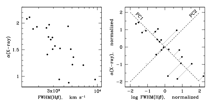 # In[3]: x=np.r_[0:8:100j] fun=[np.ones_like(x),0.5*x]#0.05*x**2] fun.append(0.3*np.sin(x*2.)) fun.append(np.exp(-(x-5)**2/2.)) fun.append(np.exp(-(x-2)**2)) nmeas=20 [pl.plot(x,f) for f in fun] pl.legend(["constant","linear","periodic","low peak","high peak"]) allpars=np.array([np.random.normal(a,0.4*abs(a),size=nmeas) for a in [3,-1,1.5,2,3.1]]) #sada ruznych koefientu jednotlivych komponent # we generate synthetic spectra by mixing 5 (non-orthogonal) functions # can be used to work in space of (physically) different variables, they should be normalized $X \to (X-E(X))/\sqrt{V(X)}$ # - now the correlation is a simple scalar product # # renfunc=testfunc-testfunc.mean(1)[:,np.newaxis] # renfunc/=np.sqrt((renfunc**2).sum(1))[:,np.newaxis] # cormat=renfunc.dot(renfunc.T) # eig,vecs=np.linalg.eig(cormat) # # in spectral analysis we look for common patterns in data (here 100 points) # - typical case: identify different materials in 2-D map # # - we have 20 sets of parameters, generate combination of 5 basic functions and add some gaussian noise # In[1]: import numpy as np nset=10 setsiz=20 nconf=4 samp1=np.random.multivariate_normal(np.zeros(nset),np.eye(nset)*0.2,setsiz).T weits=np.random.uniform(0,1,(nconf,nset)).reshape(nconf,nset,1) x=np.r_[:setsiz].reshape(1,setsiz) samp1+=weits[0]*np.sin(x*0.4+0.2) samp1+=weits[1]*np.sin(x*0.7-0.2) samp1+=weits[2]*np.sin(x*0.1+1.7) samp1+=weits[3]*(x/10.-1)*.7 get_ipython().run_line_magic('matplotlib', 'inline') from matplotlib import pyplot as plt from mpl_toolkits.mplot3d import Axes3D from mpl_toolkits.mplot3d import proj3d fig = plt.figure(figsize=(8,8)) ax = fig.add_subplot(111, projection='3d') plt.rcParams['legend.fontsize'] = 10 out=ax.plot(samp1[0,:], samp1[1,:], samp1[2,:],'o'); # In[4]: testfunc=allpars.T.dot(fun) for i in range(len(testfunc)): testfunc[i]+=np.random.normal(0,0.3,size=len(x)) pl.plot(x,testfunc[3]) pl.title("2 synthetic functions") pl.plot(x,testfunc[1]); # In[8]: renfunc=testfunc-testfunc.mean(1)[:,np.newaxis] #renormalization renfunc/=np.sqrt((renfunc**2).sum(1))[:,np.newaxis] cormat10=renfunc[:10].dot(renfunc[:10].T) eig10,vecs10=np.linalg.eig(cormat10) prinfunc=vecs10.T.dot(renfunc[:10]) [pl.plot(x,p) for p in prinfunc[:4]]; pl.title("principal functions") pl.legend(range(1,5)); # In[32]: pl.plot(range(1,11),eig10,"o-") pl.title("eigenvalues - explained variability") pl.grid() # only 3 function effectively needed # ### Lessons learned # # - most analysis tasks can be seen as *explaning variability* of experimental dataset # - reasoning for extra model parameters can be best proven by *validation* # - principal component analysis cannot separate correlated functions- but helps to reduce the information
# *... thank for your kind attention*