#!/usr/bin/env python
# coding: utf-8

# <hr style="height:2px;">
# 
# # Demo: Neural network training for combined denoising and upsamling of synthetic 3D data
# 
# This notebook demonstrates training a CARE model for a combined denoising and upsampling task, assuming that training data was already generated via [1_datagen.ipynb](1_datagen.ipynb) and has been saved to disk to the file ``data/my_training_data.npz``. Note that the training approach is exactly the same as in the standard CARE approach, what differs is the [training data generation](1_datagen.ipynb) and [prediction](3_prediction.ipynb).
# 
# Note that training a neural network for actual use should be done on more (representative) data and with more training time.
# 
# More documentation is available at http://csbdeep.bioimagecomputing.com/doc/.

# In[1]:


from __future__ import print_function, unicode_literals, absolute_import, division
import numpy as np
import matplotlib.pyplot as plt
get_ipython().run_line_magic('matplotlib', 'inline')
get_ipython().run_line_magic('config', "InlineBackend.figure_format = 'retina'")

from tifffile import imread
from csbdeep.utils import axes_dict, plot_some, plot_history
from csbdeep.utils.tf import limit_gpu_memory
from csbdeep.io import load_training_data
from csbdeep.models import Config, UpsamplingCARE


# The TensorFlow backend uses all available GPU memory by default, hence it can be useful to limit it:

# In[2]:


# limit_gpu_memory(fraction=1/2)


# <hr style="height:2px;">
# 
# # Training data
# 
# Load training data generated via [1_datagen.ipynb](1_datagen.ipynb), use 10% as validation data.

# In[3]:


(X,Y), (X_val,Y_val), axes = load_training_data('data/my_training_data.npz', validation_split=0.1, verbose=True)

c = axes_dict(axes)['C']
n_channel_in, n_channel_out = X.shape[c], Y.shape[c]


# In[4]:


plt.figure(figsize=(12,3))
plot_some(X_val[:5,...,0,0],Y_val[:5,...,0,0])
plt.suptitle('5 example validation patches (ZY slice, top row: source, bottom row: target)');


# <hr style="height:2px;">
# 
# # CARE model
# 
# Before we construct the actual CARE model, we have to define its configuration via a `Config` object, which includes 
# * parameters of the underlying neural network,
# * the learning rate,
# * the number of parameter updates per epoch,
# * the loss function, and
# * whether the model is probabilistic or not.
# 
# The defaults should be sensible in many cases, so a change should only be necessary if the training process fails.  
# 
# ---
# 
# <span style="color:red;font-weight:bold;">Important</span>: Note that for this notebook we use a very small number of update steps per epoch for immediate feedback, whereas this number should be increased considerably (e.g. `train_steps_per_epoch=400`, `train_batch_size=16`) to obtain a well-trained model.

# In[5]:


config = Config(axes, n_channel_in, n_channel_out, train_steps_per_epoch=25, train_batch_size=4)
print(config)
vars(config)


# We now create an upsampling CARE model with the chosen configuration:

# In[6]:


model = UpsamplingCARE(config, 'my_model', basedir='models')


# <hr style="height:2px;">
# 
# # Training
# 
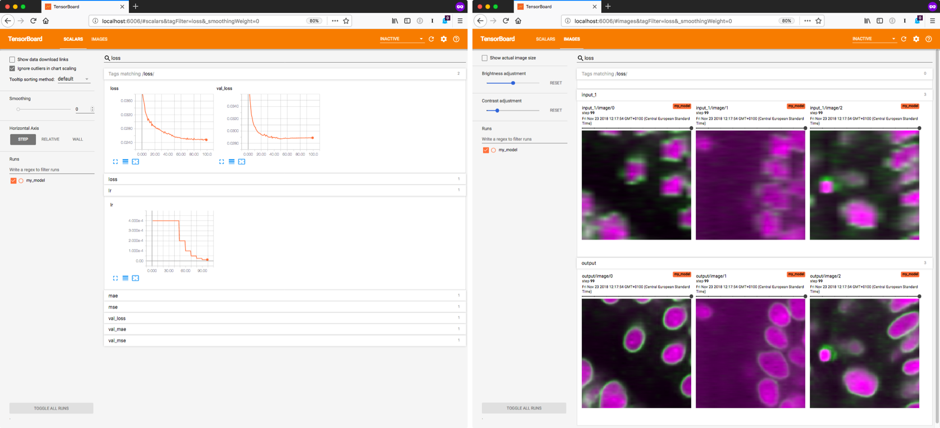
# Training the model will likely take some time. We recommend to monitor the progress with [TensorBoard](https://www.tensorflow.org/programmers_guide/summaries_and_tensorboard) (example below), which allows you to inspect the losses during training.
# Furthermore, you can look at the predictions for some of the validation images, which can be helpful to recognize problems early on.
# 
# You can start TensorBoard from the current working directory with `tensorboard --logdir=.`
# Then connect to [http://localhost:6006/](http://localhost:6006/) with your browser.
# 
# ![](http://csbdeep.bioimagecomputing.com/old/img/tensorboard_upsampling3D.png)

# In[7]:


history = model.train(X,Y, validation_data=(X_val,Y_val))


# Plot final training history (available in TensorBoard during training):

# In[8]:


print(sorted(list(history.history.keys())))
plt.figure(figsize=(16,5))
plot_history(history,['loss','val_loss'],['mse','val_mse','mae','val_mae']);


# <hr style="height:2px;">
# 
# # Evaluation
# 
# Example results for validation images.

# In[9]:


plt.figure(figsize=(12,4.5))
_P = model.keras_model.predict(X_val[:5])
if config.probabilistic:
    _P = _P[...,:(_P.shape[-1]//2)]
plot_some(X_val[:5,...,0,0],Y_val[:5,...,0,0],_P[...,0,0],pmax=99.5)
plt.suptitle('5 example validation patches (ZY slice)\n'      
             'top row: input (source),  '          
             'middle row: target (ground truth),  '
             'bottom row: predicted from source');


# <hr style="height:2px;">
# 
# # Export model to be used with CSBDeep **Fiji** plugins and **KNIME** workflows
# 
# See https://github.com/CSBDeep/CSBDeep_website/wiki/Your-Model-in-Fiji for details.

# In[10]:


model.export_TF()