#!/usr/bin/env python
# coding: utf-8

# Some more details on Floating point arithmetic discussed.
# 
# <a href="http://www-users.math.umn.edu/~arnold/disasters/">List of disasters due to bad numerical computing - I</a>
# 
# <a href="https://web.ma.utexas.edu/users/arbogast/misc/disasters.html">List of disasters due to bad numerical computing - II</a>
# $\newcommand{\magn}[1]{\lVert#1\rVert}$
# $\newcommand{\abs}[1]{\lvert#1\rvert}$
# $\newcommand{\Rb}{\mathbb{R}}$
# $\newcommand{\bkt}[1]{\left(#1\right)}$
# 
# ### Condition number
# 
# In almost all applications, we are interested in obtaining an output $f(x)$ for a given input $x$. However, there are inherent uncertainties in the input data $x$. These uncertainties could arise not only because of our inability to measure the input precisely but also due to the fact that numbers need not be represented exactly on the machine (as seen in the previous section). Hence, it is vital to understand how the solution to a problem gets affected by small perturbations in the input data. A given problem is said to be ***well-conditioned*** if "small" perturbations in $x$ result in "small" changes in $f(x)$. An ***ill-conditioned*** problem is one where "small" perturbations in $x$ lead to a "large" change in $f(x)$. The notion of "small" and "large" often depends on the problem and application of interest.
# 
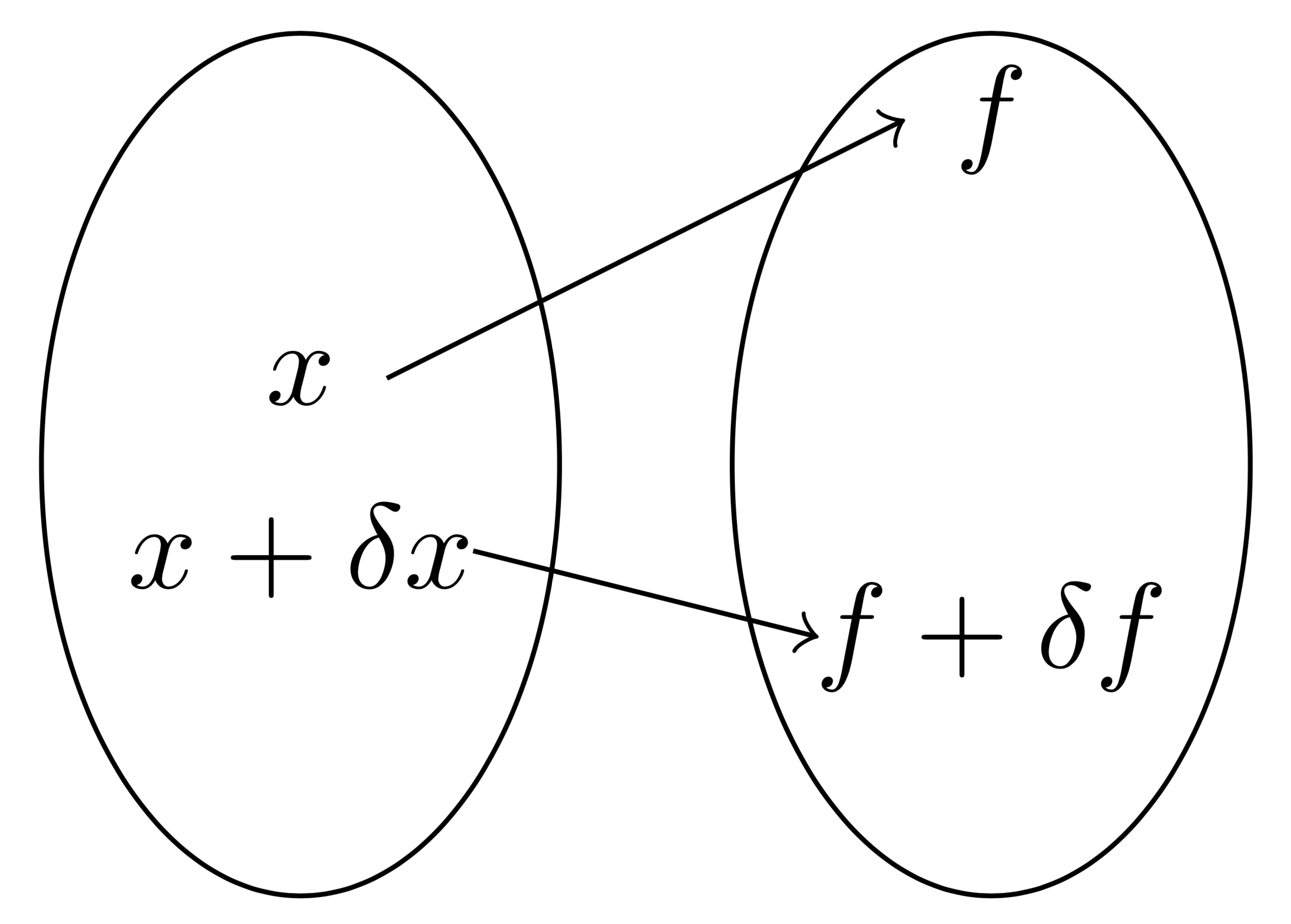# <img src="./../images/Conditioning.png" width="200" height="40">Conditioning quantifies how small/large the change $\delta f$ in output is for a $\delta x$ perturbation of the input.</img>
# 
# 
# #### Absolute condition number
# 
# One way to measure conditioning" of a problem is as follows. Let $\delta x$ denote a small perturbation of $x$ (the input) and let $\delta f = f(x+\delta x) - f(x)$ be the corresponding change in the output. The \emph{absolute condition number} $\hat{\kappa}\bkt{x,f}$ of the problem $f$ at $x$ is defined as
# $$\hat{\kappa} = \lim_{\delta \to 0} \sup_{\magn{\delta x} = \delta} \dfrac{\magn{\delta f}}{\magn{\delta x}}$$
# Note that if $f$ is differentiable at $x$, and $J(x)$ is the Jacobian of $f(x)$ at $x$, we obtain that
# $$\hat{\kappa} = \magn{J(x)}$$
# 
# #### Relative condition number
# Note that since the input ($x$) and the output ($f(x)$) are on different spaces, a more appropriate measure of conditioning is to measure the changes in the input and output in terms of relative changes. The \emph{relative condition number} $\kappa\bkt{x,f}$ of the problem $f$ at $x$ is defined as
# $$\kappa = \lim_{\delta \to 0} \sup_{\magn{\delta x} = \delta} \bkt{\dfrac{\magn{\delta f}}{\magn{f}} \bigg/ \dfrac{\magn{\delta x}}{\magn{x}}}$$
# As before, if $f$ is differentiable at $x$, we can express this in terms of the Jacobian $J(x)$ as
# $$\kappa = \dfrac{\magn{J(x)}}{\magn{f(x)}/\magn{x}}$$
# Even though both the above notions have their uses, relative condition number is more appropriate since as we saw earlier, floating point arithmetic introduces only relative errors.
# 
# #### Conditioning of subtraction
# Consider **subtracting two positive numbers**, i.e., $f(a,b) = a-b$. If we perturb $a$ by $a+\delta_a$ and $b$ by $b+\delta_b$, we have the condition number in $2$-norm to be
# $$\kappa(f,a,b) = \lim_{r \to 0} \sup_{\magn{\delta}_2 = r} \dfrac{\abs{\delta_a-\delta_b}/\abs{a-b}}{\sqrt{\delta_a^2+\delta_b^2}/\sqrt{a^2+b^2}} = \lim_{r \to 0} \sup_{\magn{\delta}_2 = r} \dfrac{\abs{\delta_a-\delta_b}/\abs{a-b}}{r/\sqrt{a^2+b^2}} = \dfrac{\sqrt{2}\sqrt{a^2+b^2}}{\abs{a-b}}$$
# Hence, we see that for large values of $a$ and $b$ such that $a-b$ is small (i.e., $a$ is close to $b$), the problem is ill-conditioned.
# 
# #### Conditioning of solving for roots of polynomials
# Consider finding the **roots of the polynomial $ax^2+bx+c$**. Here the function $f: \Rb^3 \mapsto \Rb^2$, where $f(a,b,c) = \begin{bmatrix} r_1 & r_2 \end{bmatrix}$, where $r_1,r_2$ are the roots of $ax^2+bx+c$. Now let's look at the condition at $(a,b,c) = (1,-2,1)$. The roots are $1,1$. Let's perturb the $2$ by $\delta$. We have
# \begin{align*}
# 	\kappa & = \lim_{\delta \to 0} \dfrac{\magn{f(1,-(2+\delta),1)-f(1,-2,1)}/\magn{f(1,-2,1)}}{\magn{(1,-(2+\delta),1)-(1,-2,1)}/\magn{(1,-2,1)}} = \dfrac{\magn{(1,-2,1)}}{\magn{f(1,-2,1)}}\lim_{\delta \to 0} \dfrac{\magn{\dfrac{\delta+\sqrt{\delta^2+4\delta}}2,\dfrac{\delta-\sqrt{\delta^2+4\delta}}2}}{\delta}\\
# 	& = \dfrac{\sqrt6}{2\sqrt2} \lim_{\delta \to 0} \dfrac{\sqrt{2\delta^2+2\delta^2+8\delta}}{\delta} = \sqrt3 \lim_{\delta \to 0} \dfrac{\sqrt{\delta^2+2\delta}}{\delta} = \sqrt3 \lim_{\delta \to 0} \sqrt{1+2/\delta} = \infty
# \end{align*}
# 			
# #### Conditioning of matrix-vector products
# 
# We have $f(x) = Ax$. The Jacobian is nothing but the matrix $A$. Hence, we have
# $$\kappa\bkt{x,Ax} = \dfrac{\magn{A}\magn{x}}{\magn{Ax}}$$
# Note that
# $$\magn{x} = \magn{A^{-1}\bkt{Ax}} \leq \magn{A^{-1}} \magn{Ax}$$
# Hence, we obtain that
# $$\kappa\bkt{x,Ax} = \dfrac{\magn{A}\magn{x}}{\magn{Ax}} \leq \dfrac{\magn{A}\magn{A^{-1}} \magn{Ax}}{\magn{Ax}} = \magn{A} \magn{A^{-1}}$$
# where the bound is independent of $x$. Hence, $\magn{A} \magn{A^{-1}}$ is called as the condition number of the matrix $A$ and is denoted as $\kappa(A)$.
# 
# #### Conditioning of a system of equations
# We are interested in solving the linear system $Ax=b$. In this case, we have $f(b) = A^{-1}b$. The Jacobian of $f(b)$ is nothing but the matrix $A^{-1}$. Hence, we have
# $$\kappa\bkt{b,x} = \dfrac{\magn{A^{-1}}\magn{b}}{\magn{A^{-1}b}} = \dfrac{\magn{A^{-1}}\magn{A \bkt{A^{-1}b}}}{\magn{A^{-1}b}} \leq \dfrac{\magn{A^{-1}}\magn{A} \magn{A^{-1}b}}{\magn{A^{-1}b}} = \kappa(A)$$