#!/usr/bin/env python
# coding: utf-8

# # Data Driven Modeling
# <hr style="height:3px;border:none;color:stillblue;background-color:black;" />
# ### PhD seminar series at Chair for Computer Aided Architectural Design (CAAD), ETH Zurich
# 
# 
# [Vahid Moosavi](https://vahidmoosavi.com/)
# <hr style="height:1px;border:none;color:stillblue;background-color:black;" />

# <a></a>
# 
# # Tenth Session 
# <hr style="height:1px;border:none;color:stillblue;background-color:steelblue;" />
# <span style="color:steelblue;font-size: 1em;"> 06 December 2016</span>
# 

# # Deep Networks

# ### Topics to be discussed 
# * **AutoEncoders**
# * ** Deep AutoEncoders**
# * **Representation Learning**
# * **Distributed Representation**
# * **Data Compression**

# In[80]:


import warnings
warnings.filterwarnings("ignore")
import pandas as pd
import numpy as np
from matplotlib import pyplot as plt
pd.__version__
import sys
from scipy import stats
import time
from scipy.linalg import norm
import sompylib.sompy as SOM


# we need to install tensor flow
import tensorflow as tf
import tensorflow.examples.tutorials.mnist.input_data as input_data

get_ipython().run_line_magic('matplotlib', 'inline')


# ## Review to PCA from the point of view of encoding/decoding (reconstruction)
# 

# ###  1: Encoding: X_trans = X.dot(PC)
# * **X is (Nxd) matrix, PC is a (dxd) matrix ---- > (Nxd) dot (dxd) --- > X_trans is (Nxd)**
# 
# ### 2: Decoding: X_recon = Xtrans.dot(PCs.T)
# * **X_trans is (Nxd), PC.T (dxd) --- > X_recon is (Nxd)**
# 
# 
# ## Encoding/Decoding with no compression
# ![](Images/PCA_Full.png)
# 
# ## Encoding/Decoding with  compression
# ![](Images/PCA_lower.png)
# 
# ### With this compression or dimensionality reduced encoding:
# * **We reduce the required memory**
# * ** But we loose information**

# ## Some experiments with MNIST data set and PCA

# In[82]:


"""Test the autoencoder using MNIST."""
# %%
# load MNIST as before
mnist = input_data.read_data_sets('MNIST_data', one_hot=True)
mean_img = np.mean(mnist.train.images, axis=0)


# In[63]:


import random
test_xs = mnist.test.images
test_xs_labels= mnist.test.labels
test_xs_norm = np.array([img - mean_img for img in test_xs])
import random
ind_row_test = random.sample(range(test_xs.shape[0]),500)


# In[31]:


from sklearn.decomposition import PCA
train_xs = mnist.train.images
train_xs_norm = np.array([img - mean_img for img in train_xs])
# test_xs_labels= mnist.test.labels
pca = PCA()
pca.fit(train_xs_norm)


# In[83]:


W_pca = pca.components_
W_pca.shape


# ## No dimensionality reduction
# ### No reconstruction error

# In[84]:


W_pca = pca.components_
sel_comp = W_pca.shape[1]
lowdim_PCA = test_xs_norm.dot(W_pca[:,:sel_comp])
lowdim_PCA.shape
recon_PCA = lowdim_PCA.dot(W_pca[:,:sel_comp].T)+ mean_img
n_examples = 10
fig, axs = plt.subplots(2, n_examples, figsize=(10, 2))
for example_i,ind in enumerate(ind_row_test[:n_examples]):
    axs[0][example_i].imshow(
        np.reshape(test_xs[ind, :], (28, 28)))
    axs[0][example_i].set_axis_off()
    axs[1][example_i].imshow(
            np.reshape([recon_PCA[ind, :]], (28, 28)))
    axs[1][example_i].set_axis_off()

fig.show()
plt.tight_layout()    


# ## With dimensionality reduction
# ### Reconstruction error

# In[44]:


W_pca = pca.components_
sel_comp = 400
lowdim_PCA = test_xs_norm.dot(W_pca[:,:sel_comp])
lowdim_PCA.shape
recon_PCA = lowdim_PCA.dot(W_pca[:,:sel_comp].T)+ mean_img
n_examples = 10
fig, axs = plt.subplots(2, n_examples, figsize=(10, 2))
for example_i,ind in enumerate(ind_row_test[:n_examples]):
    axs[0][example_i].imshow(
        np.reshape(test_xs[ind, :], (28, 28)))
    axs[0][example_i].set_axis_off()
    axs[1][example_i].imshow(
            np.reshape([recon_PCA[ind, :]], (28, 28)))
    axs[1][example_i].set_axis_off()

fig.show()
plt.tight_layout()    


# ## With more dimensionality reduction

# In[46]:


W_pca = pca.components_
sel_comp = 2
lowdim_PCA = test_xs_norm.dot(W_pca[:,:sel_comp])
lowdim_PCA.shape
recon_PCA = lowdim_PCA.dot(W_pca[:,:sel_comp].T)+ mean_img
n_examples = 10
fig, axs = plt.subplots(2, n_examples, figsize=(10, 2))
for example_i,ind in enumerate(ind_row_test[:n_examples]):
    axs[0][example_i].imshow(
        np.reshape(test_xs[ind, :], (28, 28)))
    axs[0][example_i].set_axis_off()
    axs[1][example_i].imshow(
            np.reshape([recon_PCA[ind, :]], (28, 28)))
    axs[1][example_i].set_axis_off()

fig.show()
plt.tight_layout()    


# ### Auto Encoders: Supervised kind of PCA reconstruction
# ![](Images/AutoEncoder.png)
# 
# 
# ![](https://wikimedia.org/api/rest_v1/media/math/render/svg/4e3bf605748634864343e8c5ffa335f301cbf955)
# 
# ![](https://wikimedia.org/api/rest_v1/media/math/render/svg/7fa0e56273a1cb32709b442e2421e9f947522b84)
# 
# 
# **elementwise activation function makes layers differentiable: https://en.wikipedia.org/wiki/Activation_function**
# 
# ![](https://wikimedia.org/api/rest_v1/media/math/render/svg/370f7b6aee47860a36b808c19582c0caaeb9c3a4)
# 
# 
# 
# **Loss function**
# ![](https://wikimedia.org/api/rest_v1/media/math/render/svg/cafbacd34534f23e90f73c0aa39fda11e29696ab)
# 
# **Backpropogarion algorithm and Stochastic gradient descent updates all the parameters after each training data**
# 

# # Deep Auto-Encoders
# #### Hinton 2006 
# https://www.cs.toronto.edu/~hinton/science.pdf
# **"It has been obvious since the 1980s that
# backpropagation through deep autoencoders
# would be very effective for nonlinear dimensionality
# reduction, provided that computers
# were fast enough, data sets were big enough,
# and the initial weights were close enough to a
# good solution. All three conditions are now
# satisfied"**
# * ** The IDEA: we take the output of first PCA and train another PCA until the last encoder layer**
# ![](Images/DeepAutoEncoder.png)
# # <a></a>

# # Professional implementations:
# ## Python libraries 
# * **TensorFlow**
# * **Theano**
# * **Keras on top of two previous ones**
# * **Lasagna on top of Theano**
# ## Other languages
# ## Torch in Lua
# ## Cafe in C++
# ## ...

# # Tensor Flow
# * https://github.com/tensorflow
# ### Introduced by Google in November 2015 

# ## Deep Autoencoders in Tensorflow

# In[49]:


"""Tutorial on how to create an autoencoder w/ Tensorflow.
Parag K. Mital, Jan 2016
"""
# %% Imports
import tensorflow as tf
import numpy as np
import math


# %% Autoencoder definition
def autoencoder(dimensions=[784, 512, 256, 64]):
    """Build a deep autoencoder w/ tied weights.
    Parameters
    ----------
    dimensions : list, optional
        The number of neurons for each layer of the autoencoder.
    Returns
    -------
    x : Tensor
        Input placeholder to the network
    z : Tensor
        Inner-most latent representation
    y : Tensor
        Output reconstruction of the input
    cost : Tensor
        Overall cost to use for training
    """
    # %% input to the network
    x = tf.placeholder(tf.float32, [None, dimensions[0]], name='x')
    current_input = x

    # %% Build the encoder
    encoder = []
    for layer_i, n_output in enumerate(dimensions[1:]):
        n_input = int(current_input.get_shape()[1])
        W = tf.Variable(
            tf.random_uniform([n_input, n_output],
                              -1.0 / math.sqrt(n_input),
                              1.0 / math.sqrt(n_input)))
        b = tf.Variable(tf.zeros([n_output]))
        encoder.append(W)
#         output = tf.nn.sigmoid(tf.matmul(current_input, W) + b)
        output = tf.nn.tanh(tf.matmul(current_input, W) + b)
        current_input = output

    # %% latent representation
    z = current_input
    encoder.reverse()

    # %% Build the decoder using the same weights
    for layer_i, n_output in enumerate(dimensions[:-1][::-1]):
        W = tf.transpose(encoder[layer_i])
        b = tf.Variable(tf.zeros([n_output]))
        output = tf.nn.tanh(tf.matmul(current_input, W) + b)
        current_input = output

    # %% now have the reconstruction through the network
    y = current_input

    # %% cost function measures pixel-wise difference
    cost = tf.reduce_sum(tf.square(y - x))
    return {'x': x, 'z': z, 'y': y, 'cost': cost}


# In[50]:


ae = autoencoder(dimensions=[784, 256, 64,2])
# ae = autoencoder(dimensions=[784,1000,500,250,2])

# %%
learning_rate = 0.001
optimizer = tf.train.AdamOptimizer(learning_rate).minimize(ae['cost'])
# %%
# We create a session to use the graph
sess = tf.Session()
sess.run(tf.initialize_all_variables())
# %%
# Fit all training data
batch_size = 50
n_epochs = 15
for epoch_i in range(n_epochs):
    for batch_i in range(mnist.train.num_examples // batch_size):
        batch_xs, _ = mnist.train.next_batch(batch_size)
        train = np.array([img - mean_img for img in batch_xs])
        sess.run(optimizer, feed_dict={ae['x']: train})
    print(epoch_i, sess.run(ae['cost'], feed_dict={ae['x']: train}))

# %%
# Plot example reconstructions
n_examples = 15
# test_xs, _ = mnist.test.next_batch(n_examples)
# test_xs_norm = np.array([img - mean_img for img in test_xs])
# recon = sess.run(ae['y'], feed_dict={ae['x']: test_xs_norm})
# fig, axs = plt.subplots(2, n_examples, figsize=(10, 2))
# for example_i in range(n_examples):
#     axs[0][example_i].imshow(
#         np.reshape(test_xs[example_i, :], (28, 28)))
#     axs[0][example_i].set_axis_off()
#     axs[1][example_i].imshow(
#             np.reshape([recon[example_i, :] + mean_img], (28, 28)))
#     axs[1][example_i].set_axis_off()

# fig.show()
# plt.draw()
# #     plt.waitforbuttonpress()



# In[64]:


recon_AE = sess.run(ae['y'], feed_dict={ae['x']: test_xs_norm})+ mean_img
lowdim_AE = sess.run(ae['z'], feed_dict={ae['x']: test_xs_norm})


# ## Comparing the results with SOM and PCA

# In[52]:


Data_tr = train_xs_norm + 1e-32*np.random.randn(train_xs_norm.shape[0],train_xs_norm.shape[1])
somMNIST = SOM.SOM('som1', Data_tr, mapsize = [60, 60],norm_method = 'var',initmethod='pca')
# som1 = SOM.SOM('som1', D, mapsize = [1, 100],norm_method = 'var',initmethod='pca')
somMNIST.train(n_job = 1, shared_memory = 'no',verbose='final')
codebook_MNIST = somMNIST.codebook[:]


# In[56]:


codebook_MNIST_n = SOM.denormalize_by(somMNIST.data_raw, codebook_MNIST, n_method = 'var') + mean_img


# In[65]:


bmu_test = somMNIST.project_data(test_xs_norm)


# In[66]:


recon_SOM = codebook_MNIST_n[bmu_test]
lowdim_SOM = somMNIST.ind_to_xy(bmu_test)


# In[67]:


lowdim_SOM.shape


# In[ ]:





# In[68]:


fig = plt.figure()
K = 9
c = np.argmax(test_xs_labels[ind_row_test],axis=1)
plt.subplot(2,2,1)
plt.scatter(lowdim_AE[ind_row_test,0],lowdim_AE[ind_row_test,1],s=50,edgecolor='None',marker='o',alpha=1.,c=plt.cm.RdYlBu_r(np.asarray(c)/float(K)));

plt.subplot(2,2,2)
plt.scatter(lowdim_PCA[ind_row_test,0],lowdim_PCA[ind_row_test,1],s=50,edgecolor='None',marker='o',alpha=1.,c=plt.cm.RdYlBu_r(np.asarray(c)/float(K)));

plt.subplot(2,2,3)
plt.scatter(lowdim_SOM[ind_row_test,0],lowdim_SOM[ind_row_test,1],s=50,edgecolor='None',marker='o',alpha=1.,c=plt.cm.RdYlBu_r(np.asarray(c)/float(K)));

fig.set_size_inches(7,7);


# In[69]:


fig, axs = plt.subplots(4, n_examples, figsize=(10, 2))
for example_i,ind in enumerate(ind_row_test[:n_examples]):
    axs[0][example_i].imshow(
        np.reshape(test_xs[ind, :], (28, 28)))
    axs[0][example_i].set_axis_off()
    axs[1][example_i].imshow(
            np.reshape([recon_PCA[ind, :]], (28, 28)))
    axs[1][example_i].set_axis_off()
    axs[2][example_i].imshow(
            np.reshape([recon_SOM[ind, :]], (28, 28)))
    axs[2][example_i].set_axis_off()
    
    axs[3][example_i].imshow(
            np.reshape([recon_AE[ind, :]], (28, 28)))
    axs[3][example_i].set_axis_off()
fig.show()
plt.draw()


# In[70]:


# %% Basic test
"""Test the autoencoder using MNIST."""
import tensorflow as tf
import tensorflow.examples.tutorials.mnist.input_data as input_data
import matplotlib.pyplot as plt

# %%
# load MNIST as before
mnist = input_data.read_data_sets('MNIST_data', one_hot=True)
mean_img = np.mean(mnist.train.images, axis=0)
ae2 = autoencoder(dimensions=[784, 256,120,80 ,64])
# ae = autoencoder(dimensions=[784,1000,500,250,2])

# %%
learning_rate = 0.001
optimizer = tf.train.AdamOptimizer(learning_rate).minimize(ae2['cost'])
# %%
# We create a session to use the graph
sess = tf.Session()
sess.run(tf.initialize_all_variables())
# %%
# Fit all training data
batch_size = 50
n_epochs = 30
for epoch_i in range(n_epochs):
    for batch_i in range(mnist.train.num_examples // batch_size):
        batch_xs, _ = mnist.train.next_batch(batch_size)
        train = np.array([img - mean_img for img in batch_xs])
        sess.run(optimizer, feed_dict={ae2['x']: train})
    print(epoch_i, sess.run(ae2['cost'], feed_dict={ae2['x']: train}))


# In[71]:


lowdim_AE2 = sess.run(ae2['z'], feed_dict={ae2['x']: test_xs_norm})
recon_AE2 = sess.run(ae2['y'], feed_dict={ae2['x']: test_xs_norm})+ mean_img


# In[72]:


somMNIST2 = SOM.SOM('som1', lowdim_AE2, mapsize = [60, 60],norm_method = 'var',initmethod='pca')
# som1 = SOM.SOM('som1', D, mapsize = [1, 100],norm_method = 'var',initmethod='pca')
somMNIST2.train(n_job = 1, shared_memory = 'no',verbose='final')
codebook_MNIST2 = somMNIST2.codebook[:]


# In[73]:


codebook_MNIST_n2 = SOM.denormalize_by(somMNIST2.data_raw, codebook_MNIST2, n_method = 'var') 


# In[74]:


bmu_test2 = somMNIST2.project_data(lowdim_AE2)


# In[75]:


recon_SOM2 = codebook_MNIST_n2[bmu_test2]
lowdim_SOM2 = somMNIST2.ind_to_xy(bmu_test2)


# In[76]:


fig = plt.figure()
K = 9
c = np.argmax(test_xs_labels[ind_row_test],axis=1)
plt.subplot(2,2,1)
plt.scatter(lowdim_AE[ind_row_test,0],lowdim_AE[ind_row_test,1],s=20,edgecolor='None',marker='o',alpha=1.,c=plt.cm.RdYlBu_r(np.asarray(c)/float(K)));

plt.subplot(2,2,2)
plt.scatter(lowdim_PCA[ind_row_test,0],lowdim_PCA[ind_row_test,1],s=20,edgecolor='None',marker='o',alpha=1.,c=plt.cm.RdYlBu_r(np.asarray(c)/float(K)));

plt.subplot(2,2,3)
plt.scatter(lowdim_SOM[ind_row_test,0],lowdim_SOM[ind_row_test,1],s=20,edgecolor='None',marker='o',alpha=1.,c=plt.cm.RdYlBu_r(np.asarray(c)/float(K)));

plt.subplot(2,2,4)
plt.scatter(lowdim_SOM2[ind_row_test,0],lowdim_SOM2[ind_row_test,1],s=20,edgecolor='None',marker='o',alpha=1.,c=plt.cm.RdYlBu_r(np.asarray(c)/float(K)));


fig.set_size_inches(7,7);


# In[79]:


fig, axs = plt.subplots(5, n_examples, figsize=(12, 4))
for example_i,ind in enumerate(ind_row_test[:n_examples]):
    axs[0][example_i].imshow(
        np.reshape(test_xs[ind, :], (28, 28)))
    axs[0][example_i].set_axis_off()
    axs[1][example_i].imshow(
            np.reshape([recon_PCA[ind, :]], (28, 28)))
    axs[1][example_i].set_axis_off()
    axs[2][example_i].imshow(
            np.reshape([recon_SOM[ind, :]], (28, 28)))
    axs[2][example_i].set_axis_off()
    axs[3][example_i].imshow(
            np.reshape([recon_AE[ind, :]], (28, 28)))
    axs[3][example_i].set_axis_off()
    axs[4][example_i].imshow(
            np.reshape([recon_AE2[ind, :]], (28, 28)))
    axs[4][example_i].set_axis_off()

    
fig.show()


# # Distributed representation: Local and non-local representation
# 
# 
# # Local representation (usually in manifold learning)
# 
# ![](http://www.cis.hut.fi/somtoolbox/theory/img1.gif)
# 
# * ** classically, each ball is one complete prototypical result**
# * ** it is very fast to learn and it is data efficient**
# * ** it works well, if we now the features of the system**
# 
# 
# # Distributed representation (Deep Learning)
# ![](http://neuralnetworksanddeeplearning.com/images/tikz41.png)
# 
# * ** each path of activations of balls along the network is one possible prototipical result**
# * ** It is a kind of distributed media or distributed memory, where elements are contributing partially**
# * ** it is slower and data hungry**
# * ** but it learns new representation, while learning to perform other task (e.g. classifications)**
# * ** by addding each layer the representational space expands exponentially**
# 

# # With similar Idea one can play with the architucture of the network
# 
# ### MLP for prediction
# ![](Images/MLP1.png)

# In[48]:


'''
A Multilayer Perceptron implementation example using TensorFlow library.
This example is using the MNIST database of handwritten digits
(http://yann.lecun.com/exdb/mnist/)
Author: Aymeric Damien
Project: https://github.com/aymericdamien/TensorFlow-Examples/
'''

# Parameters
learning_rate = 0.001
training_epochs = 20
batch_size = 100
display_step = 1

# Network Parameters
# 784-500-500-2000-10
n_hidden_1 = 500 # 1st layer number of features
n_hidden_2 = 500 # 2nd layer number of features
n_hidden_3 = 2000 # 3nd layer number of features
n_input = 784 # MNIST data input (img shape: 28*28)
n_classes = 10 # MNIST total classes (0-9 digits)

# tf Graph input
x = tf.placeholder("float", [None, n_input])
y = tf.placeholder("float", [None, n_classes])


# Create model
def multilayer_perceptron(x, weights, biases):
    # Hidden layer with RELU activation
    layer_1 = tf.add(tf.matmul(x, weights['h1']), biases['b1'])
    layer_1 = tf.nn.relu(layer_1)
    
    # Hidden layer with RELU activation
    layer_2 = tf.add(tf.matmul(layer_1, weights['h2']), biases['b2'])
    layer_2 = tf.nn.relu(layer_2)
    
    # Hidden layer with RELU activation
    layer_3 = tf.add(tf.matmul(layer_2, weights['h3']), biases['b3'])
    layer_3 = tf.nn.relu(layer_3)
    
#     # Hidden layer with RELU activation
#     layer_4 = tf.add(tf.matmul(layer_3, weights['h4']), biases['b4'])
#     layer_4 = tf.nn.relu(layer_4)

    # Output layer with linear activation
    out_layer = tf.matmul(layer_3, weights['out']) + biases['out']
    return out_layer



# In[28]:


# Store layers weight & bias
weights = {
    'h1': tf.Variable(tf.random_normal([n_input, n_hidden_1])),
    'h2': tf.Variable(tf.random_normal([n_hidden_1, n_hidden_2])),
    'h3': tf.Variable(tf.random_normal([n_hidden_2, n_hidden_3])),
#     'h4': tf.Variable(tf.random_normal([n_hidden_3, n_hidden_4])),
 
    
    'out': tf.Variable(tf.random_normal([n_hidden_3, n_classes]))
}
biases = {
    'b1': tf.Variable(tf.random_normal([n_hidden_1])),
    'b2': tf.Variable(tf.random_normal([n_hidden_2])),
    'b3': tf.Variable(tf.random_normal([n_hidden_3])),
#     'b4': tf.Variable(tf.random_normal([n_hidden_4])),
    'out': tf.Variable(tf.random_normal([n_classes]))
}

# Construct model
pred = multilayer_perceptron(x, weights, biases)

# Define loss and optimizer
cost = tf.reduce_mean(tf.nn.softmax_cross_entropy_with_logits(pred, y))
optimizer = tf.train.AdamOptimizer(learning_rate=learning_rate).minimize(cost)

# Initializing the variables
init = tf.initialize_all_variables()


# In[29]:


# Launch the graph
with tf.Session() as sess:
    sess.run(init)

    # Training cycle
    for epoch in range(training_epochs):
        avg_cost = 0.
        total_batch = int(mnist.train.num_examples/batch_size)
        # Loop over all batches
        for i in range(total_batch):
            batch_x, batch_y = mnist.train.next_batch(batch_size)
            # Run optimization op (backprop) and cost op (to get loss value)
            _, c = sess.run([optimizer, cost], feed_dict={x: batch_x,
                                                          y: batch_y})
            # Compute average loss
            avg_cost += c / total_batch
        # Display logs per epoch step
        if epoch % display_step == 0:
            print 'Epoch: {} cost:{}'.format((epoch+1), avg_cost)
    print "Optimization Finished!"

    # Test model
    correct_prediction = tf.equal(tf.argmax(pred, 1), tf.argmax(y, 1))
    # Calculate accuracy
    accuracy = tf.reduce_mean(tf.cast(correct_prediction, "float"))
    print "Accuracy:", accuracy.eval({x: mnist.test.images, y: mnist.test.labels})


# ## Nevertheless, this is not the benchmark result. There are some other tricks, which improves the results to above 99%
# * **Droup out**
# * **Convolutional Deep Networks**
# * **...**

# # Furhter examples
# * https://github.com/aymericdamien/TensorFlow-Examples
# # Tensorflow playground
# * http://playground.tensorflow.org

# # Architectural Diversity of Deep Network
# # Plug and play Machine Learning
# http://www.asimovinstitute.org/neural-network-zoo/
# 

# 
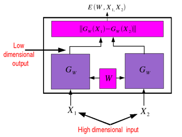
# ## Siamese network
# [Chopra,Hadsell,LeCun](https://www.cs.nyu.edu/~sumit/research/assets/cvpr05.pdf)
# ![](https://www.cs.nyu.edu/~sumit/research/files/page1_7.png)
# 
# 
# # An interesting new application:
# * Conceptually similar to Word2vec and learning contextual similarity
# * https://www.cs.cornell.edu/~sbell/pdf/siggraph2015-bell-bala.pdf