#!/usr/bin/env python
# coding: utf-8
# # Data Driven Modeling
#
# ### PhD seminar series at Chair for Computer Aided Architectural Design (CAAD), ETH Zurich
#
#
# [Vahid Moosavi](https://vahidmoosavi.com/)
#
#
#
# # Sixth Session
#
# 01 November 2016
#
# ### Topics to be discussed
#
# * **Data Clustering**
# * **K-Means**
# * **Limits and Extensions**
# * **Probabilistinc Clustering**
# * **Density based clustering**
# * **Fundamental limits to classical notion of clusters and community detection**
# * **Clustering as feature learning in comparison to PCA and sparse coding**
# * **Clustering as space indexing**
# * **Vector Quantization**
# * **Introduction to Self Organizing Maps**
#
# In[106]:
import warnings
warnings.filterwarnings("ignore")
import pandas as pd
import numpy as np
from matplotlib import pyplot as plt
pd.__version__
import sys
from scipy import stats
get_ipython().run_line_magic('matplotlib', 'inline')
# ## Data Clustering Problem
# In[107]:
# A two dimensional example
fig = plt.figure()
N = 50
d0 = 1.6*np.random.randn(N,2)
d0[:,0]= d0[:,0] - 3
plt.plot(d0[:,0],d0[:,1],'.b')
d1 = 1.6*np.random.randn(N,2)+7.6
plt.plot(d1[:,0],d1[:,1],'.b')
d2 = 1.6*np.random.randn(N,2)
d2[:,0]= d2[:,0] + 5
d2[:,1]= d2[:,1] + 1
plt.plot(d2[:,0],d2[:,1],'.b')
d3 = 1.6*np.random.randn(N,2)
d3[:,0]= d3[:,0] - 5
d3[:,1]= d3[:,1] + 4
plt.plot(d3[:,0],d3[:,1],'.b')
d4 = 1.8*np.random.randn(N,2)
d4[:,0]= d4[:,0] - 15
d4[:,1]= d4[:,1] + 14
plt.plot(d4[:,0],d4[:,1],'.b')
d5 = 1.8*np.random.randn(N,2)
d5[:,0]= d5[:,0] + 25
d5[:,1]= d5[:,1] + 14
plt.plot(d5[:,0],d5[:,1],'.b')
Data1 = np.concatenate((d0,d1,d2,d3,d4,d5))
fig.set_size_inches(7,7)
# # An important question:
# # In real scenarios why and where we have these types of clustering problems?
# * **Custormer Segmentation**
# * **Product portfolio management**
# * **Sensor placement**
# * **Location allocation problems**
# * **Understanding the (multivariate) results of several experiments**
# * **What else?**
#
# #
# In[4]:
# A two dimensional example
fig = plt.figure()
plt.plot(d0[:,0],d0[:,1],'.')
plt.plot(d1[:,0],d1[:,1],'.')
plt.plot(d2[:,0],d2[:,1],'.')
plt.plot(d3[:,0],d3[:,1],'.')
plt.plot(d4[:,0],d4[:,1],'.')
plt.plot(d5[:,0],d5[:,1],'.')
mu0= d0.mean(axis=0)[np.newaxis,:]
mu1= d1.mean(axis=0)[np.newaxis,:]
mu2= d2.mean(axis=0)[np.newaxis,:]
mu3= d3.mean(axis=0)[np.newaxis,:]
mu4= d4.mean(axis=0)[np.newaxis,:]
mu5= d5.mean(axis=0)[np.newaxis,:]
mus = np.concatenate((mu0,mu1,mu2,mu3,mu4,mu5),axis=0)
plt.plot(mus[:,0],mus[:,1],'o',markersize=10)
fig.set_size_inches(7,7)
# # K-Means clustering algorithm
#
# # Now thechnically the question in data clustering is how to get these center points?
#
#
# #
# ## Going back to the problem of regression as "energy minimization" (Least Square)
# ## $$S = \sum_{i = 1}^n ||y_i - \hat{y_i}||^2 $$
#
#
# In[108]:
N = 50
x1= np.random.normal(loc=0,scale=1,size=N)[:,np.newaxis]
x2= np.random.normal(loc=0,scale=5,size=N)[:,np.newaxis]
y = 3*x1 + np.random.normal(loc=.0, scale=.7, size=N)[:,np.newaxis]
# y = 2*x1
# y = x1*x1 + np.random.normal(loc=.0, scale=0.6, size=N)[:,np.newaxis]
# y = 2*x1*x1
fig = plt.figure(figsize=(7,7))
ax1= plt.subplot(111)
plt.plot(x1,y,'or',markersize=10,alpha=.4 );
# In[109]:
def linear_regressor(a,b):
# y_ = ax+b
mn = np.min(x1)
mx = np.max(x1)
xrng = np.linspace(mn,mx,num=500)
y_ = [a*x + b for x in xrng]
fig = plt.figure(figsize=(7,7))
ax1= plt.subplot(111)
plt.plot(x1,y,'or',markersize=10,alpha=.4 );
plt.xlabel('x1');
plt.ylabel('y');
plt.plot(xrng,y_,'-b',linewidth=1)
# plt.xlim(mn-1,mx+1)
# plt.ylim(np.min(y)+1,np.max(y)-1)
yy = [a*x + b for x in x1]
[plt.plot([x1[i],x1[i]],[yy[i],y[i]],'-r',linewidth=1) for i in range(len(x1))];
# print 'average squared error is {}'.format(np.mean((yy-y)**2))
# In[110]:
from ipywidgets import interact, HTML, FloatSlider
interact(linear_regressor,a=(-3,6,.2),b=(-2,5,.2));
# # Now look at this objective function
#  #
# ### we have $K$ centers, $\mu_i$ that create $k$ sets $S_i$ and each data point $x_i$ belongs only to one of these sets.
#
# ## In plain word, this means we need to find K vectors (n dimensional points) where, these objective function is minimum.
#
# In[111]:
import scipy.spatial.distance as DIST
def Assign_Sets(mus,X):
Dists = DIST.cdist(X,mus)
ind_sets = np.argmin(Dists,axis=1)
min_dists = np.min(Dists,axis=1)
energy = np.sum(min_dists**2)
return ind_sets, energy
def update_mus(ind_sets,X,K):
n_mus = np.zeros((K,X.shape[1]))
for k in range(K):
ind = ind_sets==k
DD = X[ind]
if DD.shape[0]>0:
n_mus[k,:]=np.mean(DD,axis=0)
else:
continue
return n_mus
def Visualize_assigned_sets(mu00=None,mu01=None,mu10=None,mu11=None,mu20=None,mu21=None):
mus0 = np.asarray([mu00,mu10,mu20])[:,np.newaxis]
mus1 = np.asarray([mu01,mu11,mu21])[:,np.newaxis]
mus = np.concatenate((mus0,mus1),axis=1)
ind_sets,energy = Assign_Sets(mus,X)
fig = plt.figure(figsize=(7,7))
ax1= plt.subplot(111)
for k,mu in enumerate(mus):
ind = ind_sets==k
DD = X[ind]
plt.plot(DD[:,0],DD[:,1],'.',markersize=10,alpha=.4 );
plt.plot(mu[0],mu[1],'ob',markersize=10,alpha=.4 );
[plt.plot([DD[i,0],mu[0]],[DD[i,1],mu[1]],'-k',linewidth=.1) for i in range(len(DD))];
# In[112]:
X = Data1.copy()
mn = np.min(X,axis=0)
mx = np.max(X,axis=0)
R = mx-mn
# Assume K = 3
from ipywidgets import interact, HTML, FloatSlider
interact(Visualize_assigned_sets,mu00=(mn[0],mx[0],1),mu01=(mn[1],mx[1],1),
mu10=(mn[0],mx[0],1),mu11=(mn[1],mx[1],1),
mu20=(mn[0],mx[0],1),mu21=(mn[1],mx[1],1));
# ## Although it looks simple, this is a hard problem and there is no exact solution for it.
# ## In order to solve this we need to use heuristic methods. For example the following steps:
# * initiate K random centers and assign each data point to its closest center.
# * Now we have K sets. Within each sets, update the location of the center to minimize the above objective function.
# * Due to the structure of these objective function, the mean vector of each set gives the minimum value.
# * Therefore, simply update the locations of center points to the mean vector of each set.
# * repeat the above steps, until the difference between two sequential centers are less than a threshhold
# In[113]:
K =5
mus_t = np.zeros((K,X.shape[1]))
mus_0 = np.zeros((K,X.shape[1]))
fig = plt.figure(figsize=(16,7));
thresh = .01
mus_0[:,0] = mn[0] + np.random.random(size=K)*R[0]
mus_0[:,1] = mn[1] + np.random.random(size=K)*R[1]
mus_t = mus_0.copy()
diff = 1000
plt.subplot(1,2,1);
plt.plot(X[:,0],X[:,1],'.');
[plt.plot(mus_t[i,0],mus_t[i,1],'or',markersize=15,linewidth=.1,label='initial') for i in range(K)];
all_diffs = []
all_energies = []
while diff> thresh:
ind_sets, energy = Assign_Sets(mus_t,X)
all_energies.append(energy)
mus_tp = update_mus(ind_sets,X,K)
diff = np.abs(mus_t- mus_tp).sum(axis=1).sum().copy()
[plt.plot([mus_t[i,0],mus_tp[i,0]],[mus_t[i,1],mus_tp[i,1]],'-og',markersize=5,linewidth=.8) for i in range(K)];
all_diffs.append(diff)
# print diff
mus_t= mus_tp.copy()
[plt.plot(mus_tp[i,0],mus_tp[i,1],'ob',markersize=15,linewidth=.1,label='final') for i in range(K)];
# # plt.legend(bbox_to_anchor=(1.1,1.));
# plt.xlabel('x');
# plt.ylabel('y');
# plt.subplot(3,1,2);
# plt.plot(all_diffs);
# plt.ylabel('average abs difference between two results');
# plt.xlabel('iterations');
plt.subplot(1,2,2);
plt.plot(all_energies,'-.r');
plt.ylabel('energy level');
plt.xlabel('iterations');
# In[114]:
def K_means(X,K):
mus_t = np.zeros((K,X.shape[1]))
mus_0 = np.zeros((K,X.shape[1]))
thresh = .01
mus_0[:,0] = mn[0] + np.random.random(size=K)*R[0]
mus_0[:,1] = mn[1] + np.random.random(size=K)*R[1]
mus_t = mus_0.copy()
diff = 1000
all_diffs = []
all_energies = []
while diff> thresh:
ind_sets, energy = Assign_Sets(mus_t,X)
all_energies.append(energy)
mus_tp = update_mus(ind_sets,X,K)
diff = np.abs(mus_t- mus_tp).sum(axis=1).sum().copy()
all_diffs.append(diff)
mus_t= mus_tp.copy()
return mus_t,all_diffs,all_energies
# # The effect of the chosen K
# In[115]:
K =5
def visualize_Kmeans(K=5):
centers, diffs, energies = K_means(X,K)
ind_sets,energy = Assign_Sets(centers,X)
fig = plt.figure()
for k in range(K):
# print
ind = ind_sets==k
DD = X[ind]
plt.plot(DD[:,0],DD[:,1],'o',alpha=0.5, markersize=4,color=plt.cm.RdYlBu_r(float(k)/K));
plt.plot(centers[k,0],centers[k,1],marker='o',markersize=15,alpha=1.,color=plt.cm.RdYlBu_r(float(k)/K));
fig.set_size_inches(7,7)
# In[116]:
from ipywidgets import interact, HTML, FloatSlider
X = Data1
interact(visualize_Kmeans,K=(1,10,1));
# # Assumptions and Extensions to K-Means
# * **How to select K in advance (metaparameter issue)**
# * **e.g. Elbow method**
# * **Similarity measures**
# * **Shape of the clusters**
# * **fuzzy k-means**
# * **Hierarchical Clustering**
# * ** Pribabilistic Clustering a.k.a Mixture Models**
# * **Sensitivity to outliers**
# * **Density based algorithms such as DBSCAN**
#
# # Probabilistic Clustering
# ## With different densities and shapes
# ### Gaussian Mixture Models
#
# * **Gaussian Mixture Model**: To learn the distribution of the data as a weighted sum of several globally defined Gaussian Distributions:
# ## $$g(X) = \sum_{i = 1}^k p_i. g(X,\theta_i)$$
# ### $ g(X,\theta_i)$ is a parametric known distribution (e.g. Gaussian) and $p_i$ is the share of each of them.
# In[117]:
import sklearn.mixture.gmm as GaussianMixture
gmm = GaussianMixture.GMM(n_components=K, random_state=0,covariance_type='full')
# In[118]:
def GMM_cluster(K=5):
from matplotlib.colors import LogNorm
import sklearn.mixture.gmm as GaussianMixture
gmm = GaussianMixture.GMM(n_components=K, random_state=0,covariance_type='full')
gmm.fit(X)
Clusters = gmm.predict(X)
fig = plt.figure()
for k in range(K):
ind = Clusters==k
DD = X[ind]
plt.plot(DD[:,0],DD[:,1],'o',alpha=1., markersize=4,color=plt.cm.RdYlBu_r(float(k)/K));
plt.plot(gmm.means_[k,0],gmm.means_[k,1],marker='o',markersize=10,alpha=1.,color=plt.cm.RdYlBu_r(float(k)/K));
# plt.plot(centers[:,0],centers[:,1],'or',alpha=1., markersize=15);
fig.set_size_inches(7,7)
x = np.linspace(X[:,0].min()-2,X[:,0].max()+2,num=200)
y = np.linspace(X[:,1].min()-2,X[:,1].max()+2,num=200)
X_, Y_ = np.meshgrid(x, y)
XX = np.array([X_.ravel(), Y_.ravel()]).T
Z = gmm.score_samples(XX)
Z = -1*Z[0].reshape(X_.shape)
# plt.imshow(Z[::-1], cmap=plt.cm.gist_earth_r,)
# plt.contour(Z[::-1])
CS = plt.contour(X_, Y_, Z, norm=LogNorm(vmin=1.0, vmax=1000.0),
levels=np.logspace(0, 3, 10),cmap=plt.cm.RdYlBu_r);
# In[119]:
from ipywidgets import interact, HTML, FloatSlider
X = Data1
pttoptdist = DIST.cdist(X,X)
interact(GMM_cluster,K=(1,6,1));
# # Assumptions and Limits to K-Means
#
# ### K-means is known to be sensitive to outliers
#
#
# # Topology Based Clustering algorithms
# # DBSCAN
# #### Density-based spatial clustering of applications with noise
#
# 
# In[120]:
def DBSCAN_1(eps=.5, MinPts=10):
Clusters = np.zeros((X.shape[0],1))
C = 1
processed = np.zeros((X.shape[0],1))
for i in range(X.shape[0]):
if processed[i]==0:
inds_neigh = pttoptdist[i]<=eps
pointers = inds_neigh*range(X.shape[0])
pointers = np.unique(pointers)[1:]
if pointers.shape[0]>= MinPts:
processed[i]==1
Clusters[i]=C
#it is a core point and not processed/clustered yet
# A new cluster
#Find other members of this cluster
counter = 0
while (counter < pointers.shape[0]):
ind = pointers[counter]
# print i,pointers.shape
if processed[ind]==0:
processed[ind] = 1
inds_neigh_C = pttoptdist[ind]<= eps
pointers_ = inds_neigh_C*range(X.shape[0])
pointers_ = np.unique(pointers_)[1:]
if pointers_.shape[0]>= MinPts:
pointers = np.concatenate((pointers,pointers_))
if Clusters[ind] == 0:
Clusters[ind] = C
counter = counter +1
C = C + 1
else:
# for now it is noise, but it might be connected later as non-core point
Clusters[i]=0
else:
continue
fig = plt.figure(figsize=(7,7))
ax1= plt.subplot(111)
K =np.unique(Clusters).shape[0]-1
for i,k in enumerate(np.unique(Clusters)[:]):
ind = Clusters==k
DD = X[ind[:,0]]
#cluster noise
if k==0:
plt.plot(DD[:,0],DD[:,1],'.k',markersize=5,alpha=1 );
else:
plt.plot(DD[:,0],DD[:,1],'o',markersize=10,alpha=.4,color=plt.cm.RdYlBu_r(float(i)/K) );
# return Clusters
# In[121]:
from ipywidgets import interact, HTML, FloatSlider
X = Data1
pttoptdist = DIST.cdist(X,X)
interact(DBSCAN_1,eps=(.05,3,.1),MinPts=(4,20,1));
# # Assumptions and Limits to K-Means
# ### shape of the clusters : K-Means classically, find spherical clusters
#
# In[122]:
dlen = 700
tetha = np.random.uniform(low=0,high=2*np.pi,size=dlen)[:,np.newaxis]
X1 = 3*np.cos(tetha)+ .22*np.random.rand(dlen,1)
Y1 = 3*np.sin(tetha)+ .22*np.random.rand(dlen,1)
D1 = np.concatenate((X1,Y1),axis=1)
X2 = 1*np.cos(tetha)+ .22*np.random.rand(dlen,1)
Y2 = 1*np.sin(tetha)+ .22*np.random.rand(dlen,1)
D2 = np.concatenate((X2,Y2),axis=1)
X3 = 5*np.cos(tetha)+ .22*np.random.rand(dlen,1)
Y3 = 5*np.sin(tetha)+ .22*np.random.rand(dlen,1)
D3 = np.concatenate((X3,Y3),axis=1)
X4 = 8*np.cos(tetha)+ .22*np.random.rand(dlen,1)
Y4 = 8*np.sin(tetha)+ .22*np.random.rand(dlen,1)
D4 = np.concatenate((X4,Y4),axis=1)
Data3 = np.concatenate((D1,D2,D3,D4),axis=0)
fig = plt.figure()
plt.plot(Data3[:,0],Data3[:,1],'ob',alpha=0.2, markersize=4)
fig.set_size_inches(7,7)
# In[123]:
from ipywidgets import interact, HTML, FloatSlider
X = Data3
interact(visualize_Kmeans,K=(1,10,1));
# In[125]:
from ipywidgets import interact, HTML, FloatSlider
X = Data3
pttoptdist = DIST.cdist(X,X)
interact(DBSCAN_1,eps=(.1,2,.1),MinPts=(4,20,1));
# # However, since DBSCAN has it own limit: It assumes a global ratio for density
# In[126]:
# A two dimensional example
fig = plt.figure()
N = 280
d0 = .5*np.random.randn(N,2) + [[3,2]]
d0 = .5*np.random.multivariate_normal([3,2],[[.8,.6],[.71,.7]],N)
plt.plot(d0[:,0],d0[:,1],'.b')
d1 = .6*np.random.randn(1*N,2)
plt.plot(d1[:,0],d1[:,1],'.b')
d2 = .5*np.random.randn(2*N,2)+[[-3,2]]
plt.plot(d2[:,0],d2[:,1],'.b')
# d3 = 1.6*np.random.randn(N,2)
# d3[:,0]= d3[:,0] - 5
# d3[:,1]= d3[:,1] + 4
# plt.plot(d3[:,0],d3[:,1],'.b')
Data2 = np.concatenate((d0,d1,d2))
fig.set_size_inches(7,7)
# In[128]:
from ipywidgets import interact, HTML, FloatSlider
X = Data2
pttoptdist = DIST.cdist(X,X)
interact(DBSCAN_1,eps=(.05,3,.05),MinPts=(4,20,1));
# In[129]:
from ipywidgets import interact, HTML, FloatSlider
X = Data2
interact(visualize_Kmeans,K=(1,3,1));
# # More than that, topological algorithms like DBSCAN have fundamental limits:
# ## They are usually developed based on synthetic data sets, which usually never happens in reality
# ## Further, they believe in some kind of underlying true groups!!! Or some kind of Idealized set up such as having perfect communities!!!
# #
# # More Important: They have NO data Abstraction and NO Generalization
#
# # Attention to these issues can be a turining point in the notion of clustering
#
# #
#
# #
# #
#
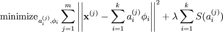
# # A different use of K-Means and its abstraction
#
# ## Clustering as Feature Transformation and Dictionary Learning
# # If we look at K-means ojective function
# 
#
# ## In comparison to Sparse Coding (SC) objective function
# 
#
#
# ### Or to PCA
#
# ## $$ x = yP $$
#
# ### Or to GMM
# ## $$g(X) = \sum_{i = 1}^k p_i. g(X,\theta_i)$$
#
# # We can think of cluster centers as new "fictional" dimensions.
# ## Then, similar to PCA or SC, the identified cluster centers can be used as dimensionality of the data points.
# ## Previous floor plan example that we had with PCA and SC
# In[76]:
from sklearn.datasets import fetch_mldata
from sklearn.datasets import fetch_olivetti_faces
#Chairs
path = "./Data/chairs.csv"
D = pd.read_csv(path,header=None)
image_shape = (64,64)
Images = D.values[:]
print Images.shape
# floorplan
path = "./Data/1000FloorPlans.csv"
D = pd.read_csv(path,header=None)
image_shape = (50, 50)
faces = D.values[:]
# faces[faces>0] = -1
# faces[faces==0] = 1
# faces[faces==-1] = 0
Images = faces[:]
print Images.shape
# # Mnist data set
# image_shape = (28, 28)
# dataset = fetch_mldata('MNIST original')
# # faces = dataset.data
# X = faces[:]
# X.shape
fig = plt.figure(figsize=(12,12))
for i in range(25):
plt.subplot(5,5,i+1)
plt.imshow(Images[i].reshape(image_shape),cmap=plt.cm.gray);
plt.xticks([]);
plt.yticks([]);
plt.tight_layout()
# In[77]:
from sklearn.feature_extraction.image import extract_patches_2d
rng = np.random.RandomState(0)
patch_size = (16, 16)
buffer = []
for img in Images:
data = extract_patches_2d(img.reshape(image_shape), patch_size, max_patches=50,
random_state=rng)
data = np.reshape(data, (len(data), -1))
buffer.extend(data)
Patch_Images = np.asarray(buffer)
print Patch_Images.shape
# In[78]:
fig = plt.figure(figsize=(12,12))
for i in range(25):
plt.subplot(5,5,i+1)
plt.imshow(Patch_Images[1000+i].reshape(patch_size),cmap=plt.cm.gray);
plt.xticks([]);
plt.yticks([]);
plt.tight_layout()
# In[79]:
means = Patch_Images.mean(axis=1)[:,np.newaxis]
Vars = Patch_Images.std(axis=1)**2 +.05
denom = np.sqrt(Vars)[:,np.newaxis]
Patch_Images = (Patch_Images-means)/denom
# /
# In[84]:
from sklearn.cluster import KMeans
kmeans = KMeans(n_clusters=200, random_state=0).fit(Patch_Images)
# In[85]:
fig = plt.figure(figsize=(10,20))
for i in range(200):
plt.subplot(20,10,i+1)
plt.imshow(kmeans.cluster_centers_[i,:].reshape(patch_size),cmap=plt.cm.gray);
plt.xticks([]);
plt.yticks([]);
plt.tight_layout(h_pad=.01, w_pad=.01)
# # Later these features can be used for classification or prediction purposes
# # We discuss them in one of the next sessions on Classification
# ### Further reading
# * https://cs.stanford.edu/~acoates/papers/coatesng_nntot2012.pdf
# # Another view to the problem of clustering
#
#
# ## Are outliers bad things or good things?
#
# ### Examples:
# * **research communities and those research topics that don't belong to any group?**
# * ** Can we say outliers might be those who are ahead of their fields?
# * ** What if we set our criteria based on the above clustering definition?**
#
# * ** One tricky recent application of ML in peer review process: Quick pre-assessments of papers for their potential popularity!!!***
# http://www.ariessys.com/views-press/press-releases/artificial-intelligence-integration-allows-publishers-first-look-meta-bibliometric-intelligence/
#
#
#
#
# # What if we say each obsevation is a potential communiy itself?
#
#
#
# # What if we increase K in K-means drastically
# In[130]:
from ipywidgets import interact, HTML, FloatSlider
X = Data3
interact(visualize_Kmeans,K=(3,300,1));
# In[131]:
from ipywidgets import interact, HTML, FloatSlider
X = Data1
interact(visualize_Kmeans,K=(200,300,1));
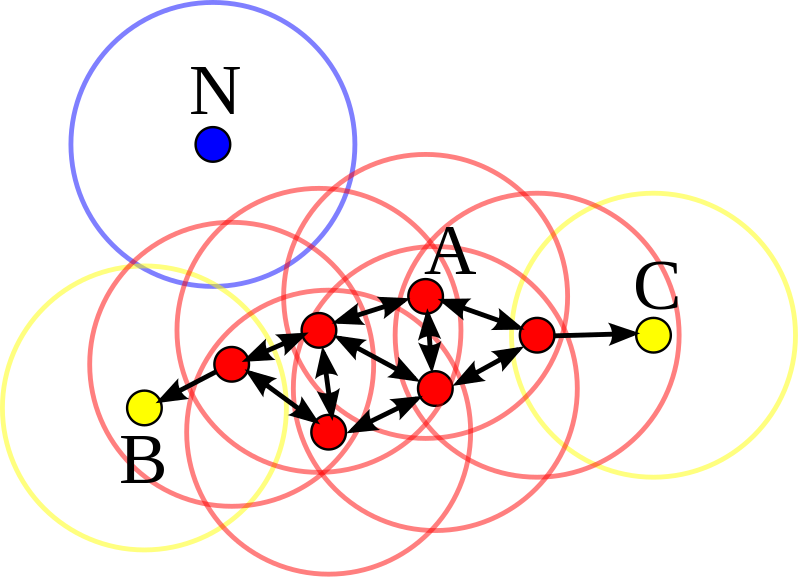
# # This is the origin of the idea of Vector Quantization.
# ### However, K-means is not scaling perfectly. For example, most of clusters overlap.
# #
#
# # If we look at it as a kind of indexing of the space, we need to sort the indices themselve!
# # In order to do so, we invert the whole game of data clustering
# # we create an aribitrary ordered set of indexes and try to fit them to data, while having a "topology preserving" indexing.
#
# # This means, if two indices have similar label, they should index a similar area of data space and vice versa.
#
# # This is the original idea of Self Organizing Maps (SOM)
# In[137]:
import sompylib.sompy as SOM
msz11 =15
msz10 = 10
X = Data1
som1 = SOM.SOM('', X, mapsize = [msz10, msz11],norm_method = 'var',initmethod='random')
som1.init_map()
som1.train(n_job = 1, shared_memory = 'no',verbose='final')
codebook1 = som1.codebook[:]
codebook1_n = SOM.denormalize_by(som1.data_raw, codebook1, n_method = 'var')
# In[138]:
fig = plt.figure()
plt.plot(X[:,0],X[:,1],'ok',alpha=0.5, markersize=4);
K = som1.nnodes
for k in range(som1.nnodes):
plt.plot(codebook1_n[k,0],codebook1_n[k,1],marker='o',markersize=10,alpha=1.,color=plt.cm.RdYlBu_r(float(k)/K));
fig.set_size_inches(7,7)
# In[139]:
som1.hit_map()
# In[140]:
som1.view_map(text_size=6,COL_SiZe=4)
#
# # This mechanism of indexing the space is called manifold learning and as we will see later SOM has lots of amazing capacities for many hig-dimensioanl data sets.
#
# # An example with high dimensional data
# In[141]:
path = "./Data/rentalprice.csv"
D = pd.read_csv(path)
# D = D[['Rent','ZIP','Year built','Living space','lng','lat']]
D.head()
# In[ ]:
# In[142]:
import sompylib.sompy as SOM
msz11 =40
msz10 = 40
X = D.values[:]
som1 = SOM.SOM('', X, mapsize = [msz10, msz11],norm_method = 'var',initmethod='pca')
som1.init_map()
som1.train(n_job = 1, shared_memory = 'no',verbose='final')
codebook1 = som1.codebook[:]
codebook1_n = SOM.denormalize_by(som1.data_raw, codebook1, n_method = 'var')
som1.compname= [D.columns]
# In[143]:
som1.hit_map()
# In[ ]:
# In[144]:
som1.view_map(text_size=6,COL_SiZe=4)
# # How this inverts the notion of clustering and detection of communities and their outliers to the communities around individuals!
# In[145]:
N = 50
x1= np.random.normal(loc=17,scale=5,size=N)[:,np.newaxis]
x2= np.random.normal(loc=0,scale=10,size=N)[:,np.newaxis]
y = 3*x1 + np.random.normal(loc=.0, scale=.4, size=N)[:,np.newaxis]
# x1 = np.random.uniform(size=N)[:,np.newaxis]
# y = np.sin(2*np.pi*x1**3)**3 + .1*np.random.randn(*x1.shape)
y =-.1*x1**3 + 2*x1*x1 + 2*np.sqrt(x1)+ 10*np.random.normal(loc=30.0, scale=4.7, size=len(x1))[:,np.newaxis]
degree= 2
from sklearn.preprocessing import PolynomialFeatures
from sklearn import linear_model
X_tr = x1[:].astype(float)
y_tr = y[:].astype(float)
poly = PolynomialFeatures(degree=degree)
X_tr_ = poly.fit_transform(X_tr)
regr = linear_model.LinearRegression()
regr.fit(X_tr_, y_tr)
X_pred = np.linspace(X_tr.min(),X_tr.max(),num=500)[:,np.newaxis]
X_pred_ = poly.fit_transform(X_pred)
y_pred = regr.predict(X_pred_)[:]
# In[146]:
import sompylib.sompy as SOM
msz11 =20
msz10 = 20
X = np.concatenate((x1,y),axis=1)
som1 = SOM.SOM('', X, mapsize = [msz10, msz11],norm_method = 'var',initmethod='pca')
som1.init_map()
som1.train(n_job = 1, shared_memory = 'no',verbose='final')
codebook1 = som1.codebook[:]
codebook1_n = SOM.denormalize_by(som1.data_raw, codebook1, n_method = 'var')
# In[147]:
fig = plt.figure()
fig.set_size_inches(14,7)
plt.subplot(1,2,1)
plt.title('data points vote for the line')
plt.plot(X_tr,y_tr,'.r',markersize=20,alpha=.4 );
plt.plot(X_pred,y_pred,'ok',markersize=3,alpha=.4 );
plt.subplot(1,2,2)
plt.title('each data point creates its own community')
plt.plot(X[:,0],X[:,1],'.r',alpha=0.5, markersize=20);
plt.plot(codebook1_n[:,0],codebook1_n[:,1],'ok',markersize=3,alpha=1.);
plt.tight_layout()
font = {'size' : 12}
plt.rc('font', **font)
# # Next session we discuss SOM and its applications
#
# ### we have $K$ centers, $\mu_i$ that create $k$ sets $S_i$ and each data point $x_i$ belongs only to one of these sets.
#
# ## In plain word, this means we need to find K vectors (n dimensional points) where, these objective function is minimum.
#
# In[111]:
import scipy.spatial.distance as DIST
def Assign_Sets(mus,X):
Dists = DIST.cdist(X,mus)
ind_sets = np.argmin(Dists,axis=1)
min_dists = np.min(Dists,axis=1)
energy = np.sum(min_dists**2)
return ind_sets, energy
def update_mus(ind_sets,X,K):
n_mus = np.zeros((K,X.shape[1]))
for k in range(K):
ind = ind_sets==k
DD = X[ind]
if DD.shape[0]>0:
n_mus[k,:]=np.mean(DD,axis=0)
else:
continue
return n_mus
def Visualize_assigned_sets(mu00=None,mu01=None,mu10=None,mu11=None,mu20=None,mu21=None):
mus0 = np.asarray([mu00,mu10,mu20])[:,np.newaxis]
mus1 = np.asarray([mu01,mu11,mu21])[:,np.newaxis]
mus = np.concatenate((mus0,mus1),axis=1)
ind_sets,energy = Assign_Sets(mus,X)
fig = plt.figure(figsize=(7,7))
ax1= plt.subplot(111)
for k,mu in enumerate(mus):
ind = ind_sets==k
DD = X[ind]
plt.plot(DD[:,0],DD[:,1],'.',markersize=10,alpha=.4 );
plt.plot(mu[0],mu[1],'ob',markersize=10,alpha=.4 );
[plt.plot([DD[i,0],mu[0]],[DD[i,1],mu[1]],'-k',linewidth=.1) for i in range(len(DD))];
# In[112]:
X = Data1.copy()
mn = np.min(X,axis=0)
mx = np.max(X,axis=0)
R = mx-mn
# Assume K = 3
from ipywidgets import interact, HTML, FloatSlider
interact(Visualize_assigned_sets,mu00=(mn[0],mx[0],1),mu01=(mn[1],mx[1],1),
mu10=(mn[0],mx[0],1),mu11=(mn[1],mx[1],1),
mu20=(mn[0],mx[0],1),mu21=(mn[1],mx[1],1));
# ## Although it looks simple, this is a hard problem and there is no exact solution for it.
# ## In order to solve this we need to use heuristic methods. For example the following steps:
# * initiate K random centers and assign each data point to its closest center.
# * Now we have K sets. Within each sets, update the location of the center to minimize the above objective function.
# * Due to the structure of these objective function, the mean vector of each set gives the minimum value.
# * Therefore, simply update the locations of center points to the mean vector of each set.
# * repeat the above steps, until the difference between two sequential centers are less than a threshhold
# In[113]:
K =5
mus_t = np.zeros((K,X.shape[1]))
mus_0 = np.zeros((K,X.shape[1]))
fig = plt.figure(figsize=(16,7));
thresh = .01
mus_0[:,0] = mn[0] + np.random.random(size=K)*R[0]
mus_0[:,1] = mn[1] + np.random.random(size=K)*R[1]
mus_t = mus_0.copy()
diff = 1000
plt.subplot(1,2,1);
plt.plot(X[:,0],X[:,1],'.');
[plt.plot(mus_t[i,0],mus_t[i,1],'or',markersize=15,linewidth=.1,label='initial') for i in range(K)];
all_diffs = []
all_energies = []
while diff> thresh:
ind_sets, energy = Assign_Sets(mus_t,X)
all_energies.append(energy)
mus_tp = update_mus(ind_sets,X,K)
diff = np.abs(mus_t- mus_tp).sum(axis=1).sum().copy()
[plt.plot([mus_t[i,0],mus_tp[i,0]],[mus_t[i,1],mus_tp[i,1]],'-og',markersize=5,linewidth=.8) for i in range(K)];
all_diffs.append(diff)
# print diff
mus_t= mus_tp.copy()
[plt.plot(mus_tp[i,0],mus_tp[i,1],'ob',markersize=15,linewidth=.1,label='final') for i in range(K)];
# # plt.legend(bbox_to_anchor=(1.1,1.));
# plt.xlabel('x');
# plt.ylabel('y');
# plt.subplot(3,1,2);
# plt.plot(all_diffs);
# plt.ylabel('average abs difference between two results');
# plt.xlabel('iterations');
plt.subplot(1,2,2);
plt.plot(all_energies,'-.r');
plt.ylabel('energy level');
plt.xlabel('iterations');
# In[114]:
def K_means(X,K):
mus_t = np.zeros((K,X.shape[1]))
mus_0 = np.zeros((K,X.shape[1]))
thresh = .01
mus_0[:,0] = mn[0] + np.random.random(size=K)*R[0]
mus_0[:,1] = mn[1] + np.random.random(size=K)*R[1]
mus_t = mus_0.copy()
diff = 1000
all_diffs = []
all_energies = []
while diff> thresh:
ind_sets, energy = Assign_Sets(mus_t,X)
all_energies.append(energy)
mus_tp = update_mus(ind_sets,X,K)
diff = np.abs(mus_t- mus_tp).sum(axis=1).sum().copy()
all_diffs.append(diff)
mus_t= mus_tp.copy()
return mus_t,all_diffs,all_energies
# # The effect of the chosen K
# In[115]:
K =5
def visualize_Kmeans(K=5):
centers, diffs, energies = K_means(X,K)
ind_sets,energy = Assign_Sets(centers,X)
fig = plt.figure()
for k in range(K):
# print
ind = ind_sets==k
DD = X[ind]
plt.plot(DD[:,0],DD[:,1],'o',alpha=0.5, markersize=4,color=plt.cm.RdYlBu_r(float(k)/K));
plt.plot(centers[k,0],centers[k,1],marker='o',markersize=15,alpha=1.,color=plt.cm.RdYlBu_r(float(k)/K));
fig.set_size_inches(7,7)
# In[116]:
from ipywidgets import interact, HTML, FloatSlider
X = Data1
interact(visualize_Kmeans,K=(1,10,1));
# # Assumptions and Extensions to K-Means
# * **How to select K in advance (metaparameter issue)**
# * **e.g. Elbow method**
# * **Similarity measures**
# * **Shape of the clusters**
# * **fuzzy k-means**
# * **Hierarchical Clustering**
# * ** Pribabilistic Clustering a.k.a Mixture Models**
# * **Sensitivity to outliers**
# * **Density based algorithms such as DBSCAN**
#
# # Probabilistic Clustering
# ## With different densities and shapes
# ### Gaussian Mixture Models
#
# * **Gaussian Mixture Model**: To learn the distribution of the data as a weighted sum of several globally defined Gaussian Distributions:
# ## $$g(X) = \sum_{i = 1}^k p_i. g(X,\theta_i)$$
# ### $ g(X,\theta_i)$ is a parametric known distribution (e.g. Gaussian) and $p_i$ is the share of each of them.
# In[117]:
import sklearn.mixture.gmm as GaussianMixture
gmm = GaussianMixture.GMM(n_components=K, random_state=0,covariance_type='full')
# In[118]:
def GMM_cluster(K=5):
from matplotlib.colors import LogNorm
import sklearn.mixture.gmm as GaussianMixture
gmm = GaussianMixture.GMM(n_components=K, random_state=0,covariance_type='full')
gmm.fit(X)
Clusters = gmm.predict(X)
fig = plt.figure()
for k in range(K):
ind = Clusters==k
DD = X[ind]
plt.plot(DD[:,0],DD[:,1],'o',alpha=1., markersize=4,color=plt.cm.RdYlBu_r(float(k)/K));
plt.plot(gmm.means_[k,0],gmm.means_[k,1],marker='o',markersize=10,alpha=1.,color=plt.cm.RdYlBu_r(float(k)/K));
# plt.plot(centers[:,0],centers[:,1],'or',alpha=1., markersize=15);
fig.set_size_inches(7,7)
x = np.linspace(X[:,0].min()-2,X[:,0].max()+2,num=200)
y = np.linspace(X[:,1].min()-2,X[:,1].max()+2,num=200)
X_, Y_ = np.meshgrid(x, y)
XX = np.array([X_.ravel(), Y_.ravel()]).T
Z = gmm.score_samples(XX)
Z = -1*Z[0].reshape(X_.shape)
# plt.imshow(Z[::-1], cmap=plt.cm.gist_earth_r,)
# plt.contour(Z[::-1])
CS = plt.contour(X_, Y_, Z, norm=LogNorm(vmin=1.0, vmax=1000.0),
levels=np.logspace(0, 3, 10),cmap=plt.cm.RdYlBu_r);
# In[119]:
from ipywidgets import interact, HTML, FloatSlider
X = Data1
pttoptdist = DIST.cdist(X,X)
interact(GMM_cluster,K=(1,6,1));
# # Assumptions and Limits to K-Means
#
# ### K-means is known to be sensitive to outliers
#
#
# # Topology Based Clustering algorithms
# # DBSCAN
# #### Density-based spatial clustering of applications with noise
#
# 
# In[120]:
def DBSCAN_1(eps=.5, MinPts=10):
Clusters = np.zeros((X.shape[0],1))
C = 1
processed = np.zeros((X.shape[0],1))
for i in range(X.shape[0]):
if processed[i]==0:
inds_neigh = pttoptdist[i]<=eps
pointers = inds_neigh*range(X.shape[0])
pointers = np.unique(pointers)[1:]
if pointers.shape[0]>= MinPts:
processed[i]==1
Clusters[i]=C
#it is a core point and not processed/clustered yet
# A new cluster
#Find other members of this cluster
counter = 0
while (counter < pointers.shape[0]):
ind = pointers[counter]
# print i,pointers.shape
if processed[ind]==0:
processed[ind] = 1
inds_neigh_C = pttoptdist[ind]<= eps
pointers_ = inds_neigh_C*range(X.shape[0])
pointers_ = np.unique(pointers_)[1:]
if pointers_.shape[0]>= MinPts:
pointers = np.concatenate((pointers,pointers_))
if Clusters[ind] == 0:
Clusters[ind] = C
counter = counter +1
C = C + 1
else:
# for now it is noise, but it might be connected later as non-core point
Clusters[i]=0
else:
continue
fig = plt.figure(figsize=(7,7))
ax1= plt.subplot(111)
K =np.unique(Clusters).shape[0]-1
for i,k in enumerate(np.unique(Clusters)[:]):
ind = Clusters==k
DD = X[ind[:,0]]
#cluster noise
if k==0:
plt.plot(DD[:,0],DD[:,1],'.k',markersize=5,alpha=1 );
else:
plt.plot(DD[:,0],DD[:,1],'o',markersize=10,alpha=.4,color=plt.cm.RdYlBu_r(float(i)/K) );
# return Clusters
# In[121]:
from ipywidgets import interact, HTML, FloatSlider
X = Data1
pttoptdist = DIST.cdist(X,X)
interact(DBSCAN_1,eps=(.05,3,.1),MinPts=(4,20,1));
# # Assumptions and Limits to K-Means
# ### shape of the clusters : K-Means classically, find spherical clusters
#
# In[122]:
dlen = 700
tetha = np.random.uniform(low=0,high=2*np.pi,size=dlen)[:,np.newaxis]
X1 = 3*np.cos(tetha)+ .22*np.random.rand(dlen,1)
Y1 = 3*np.sin(tetha)+ .22*np.random.rand(dlen,1)
D1 = np.concatenate((X1,Y1),axis=1)
X2 = 1*np.cos(tetha)+ .22*np.random.rand(dlen,1)
Y2 = 1*np.sin(tetha)+ .22*np.random.rand(dlen,1)
D2 = np.concatenate((X2,Y2),axis=1)
X3 = 5*np.cos(tetha)+ .22*np.random.rand(dlen,1)
Y3 = 5*np.sin(tetha)+ .22*np.random.rand(dlen,1)
D3 = np.concatenate((X3,Y3),axis=1)
X4 = 8*np.cos(tetha)+ .22*np.random.rand(dlen,1)
Y4 = 8*np.sin(tetha)+ .22*np.random.rand(dlen,1)
D4 = np.concatenate((X4,Y4),axis=1)
Data3 = np.concatenate((D1,D2,D3,D4),axis=0)
fig = plt.figure()
plt.plot(Data3[:,0],Data3[:,1],'ob',alpha=0.2, markersize=4)
fig.set_size_inches(7,7)
# In[123]:
from ipywidgets import interact, HTML, FloatSlider
X = Data3
interact(visualize_Kmeans,K=(1,10,1));
# In[125]:
from ipywidgets import interact, HTML, FloatSlider
X = Data3
pttoptdist = DIST.cdist(X,X)
interact(DBSCAN_1,eps=(.1,2,.1),MinPts=(4,20,1));
# # However, since DBSCAN has it own limit: It assumes a global ratio for density
# In[126]:
# A two dimensional example
fig = plt.figure()
N = 280
d0 = .5*np.random.randn(N,2) + [[3,2]]
d0 = .5*np.random.multivariate_normal([3,2],[[.8,.6],[.71,.7]],N)
plt.plot(d0[:,0],d0[:,1],'.b')
d1 = .6*np.random.randn(1*N,2)
plt.plot(d1[:,0],d1[:,1],'.b')
d2 = .5*np.random.randn(2*N,2)+[[-3,2]]
plt.plot(d2[:,0],d2[:,1],'.b')
# d3 = 1.6*np.random.randn(N,2)
# d3[:,0]= d3[:,0] - 5
# d3[:,1]= d3[:,1] + 4
# plt.plot(d3[:,0],d3[:,1],'.b')
Data2 = np.concatenate((d0,d1,d2))
fig.set_size_inches(7,7)
# In[128]:
from ipywidgets import interact, HTML, FloatSlider
X = Data2
pttoptdist = DIST.cdist(X,X)
interact(DBSCAN_1,eps=(.05,3,.05),MinPts=(4,20,1));
# In[129]:
from ipywidgets import interact, HTML, FloatSlider
X = Data2
interact(visualize_Kmeans,K=(1,3,1));
# # More than that, topological algorithms like DBSCAN have fundamental limits:
# ## They are usually developed based on synthetic data sets, which usually never happens in reality
# ## Further, they believe in some kind of underlying true groups!!! Or some kind of Idealized set up such as having perfect communities!!!
# #
# # More Important: They have NO data Abstraction and NO Generalization
#
# # Attention to these issues can be a turining point in the notion of clustering
#
# #
#
# #
# #
#
# # A different use of K-Means and its abstraction
#
# ## Clustering as Feature Transformation and Dictionary Learning
# # If we look at K-means ojective function
# 
#
# ## In comparison to Sparse Coding (SC) objective function
# 
#
#
# ### Or to PCA
#
# ## $$ x = yP $$
#
# ### Or to GMM
# ## $$g(X) = \sum_{i = 1}^k p_i. g(X,\theta_i)$$
#
# # We can think of cluster centers as new "fictional" dimensions.
# ## Then, similar to PCA or SC, the identified cluster centers can be used as dimensionality of the data points.
# ## Previous floor plan example that we had with PCA and SC
# In[76]:
from sklearn.datasets import fetch_mldata
from sklearn.datasets import fetch_olivetti_faces
#Chairs
path = "./Data/chairs.csv"
D = pd.read_csv(path,header=None)
image_shape = (64,64)
Images = D.values[:]
print Images.shape
# floorplan
path = "./Data/1000FloorPlans.csv"
D = pd.read_csv(path,header=None)
image_shape = (50, 50)
faces = D.values[:]
# faces[faces>0] = -1
# faces[faces==0] = 1
# faces[faces==-1] = 0
Images = faces[:]
print Images.shape
# # Mnist data set
# image_shape = (28, 28)
# dataset = fetch_mldata('MNIST original')
# # faces = dataset.data
# X = faces[:]
# X.shape
fig = plt.figure(figsize=(12,12))
for i in range(25):
plt.subplot(5,5,i+1)
plt.imshow(Images[i].reshape(image_shape),cmap=plt.cm.gray);
plt.xticks([]);
plt.yticks([]);
plt.tight_layout()
# In[77]:
from sklearn.feature_extraction.image import extract_patches_2d
rng = np.random.RandomState(0)
patch_size = (16, 16)
buffer = []
for img in Images:
data = extract_patches_2d(img.reshape(image_shape), patch_size, max_patches=50,
random_state=rng)
data = np.reshape(data, (len(data), -1))
buffer.extend(data)
Patch_Images = np.asarray(buffer)
print Patch_Images.shape
# In[78]:
fig = plt.figure(figsize=(12,12))
for i in range(25):
plt.subplot(5,5,i+1)
plt.imshow(Patch_Images[1000+i].reshape(patch_size),cmap=plt.cm.gray);
plt.xticks([]);
plt.yticks([]);
plt.tight_layout()
# In[79]:
means = Patch_Images.mean(axis=1)[:,np.newaxis]
Vars = Patch_Images.std(axis=1)**2 +.05
denom = np.sqrt(Vars)[:,np.newaxis]
Patch_Images = (Patch_Images-means)/denom
# /
# In[84]:
from sklearn.cluster import KMeans
kmeans = KMeans(n_clusters=200, random_state=0).fit(Patch_Images)
# In[85]:
fig = plt.figure(figsize=(10,20))
for i in range(200):
plt.subplot(20,10,i+1)
plt.imshow(kmeans.cluster_centers_[i,:].reshape(patch_size),cmap=plt.cm.gray);
plt.xticks([]);
plt.yticks([]);
plt.tight_layout(h_pad=.01, w_pad=.01)
# # Later these features can be used for classification or prediction purposes
# # We discuss them in one of the next sessions on Classification
# ### Further reading
# * https://cs.stanford.edu/~acoates/papers/coatesng_nntot2012.pdf
# # Another view to the problem of clustering
#
#
# ## Are outliers bad things or good things?
#
# ### Examples:
# * **research communities and those research topics that don't belong to any group?**
# * ** Can we say outliers might be those who are ahead of their fields?
# * ** What if we set our criteria based on the above clustering definition?**
#
# * ** One tricky recent application of ML in peer review process: Quick pre-assessments of papers for their potential popularity!!!***
# http://www.ariessys.com/views-press/press-releases/artificial-intelligence-integration-allows-publishers-first-look-meta-bibliometric-intelligence/
#
#
#
#
# # What if we say each obsevation is a potential communiy itself?
#
#
#
# # What if we increase K in K-means drastically
# In[130]:
from ipywidgets import interact, HTML, FloatSlider
X = Data3
interact(visualize_Kmeans,K=(3,300,1));
# In[131]:
from ipywidgets import interact, HTML, FloatSlider
X = Data1
interact(visualize_Kmeans,K=(200,300,1));
# # This is the origin of the idea of Vector Quantization.
# ### However, K-means is not scaling perfectly. For example, most of clusters overlap.
# #
#
# # If we look at it as a kind of indexing of the space, we need to sort the indices themselve!
# # In order to do so, we invert the whole game of data clustering
# # we create an aribitrary ordered set of indexes and try to fit them to data, while having a "topology preserving" indexing.
#
# # This means, if two indices have similar label, they should index a similar area of data space and vice versa.
#
# # This is the original idea of Self Organizing Maps (SOM)
# In[137]:
import sompylib.sompy as SOM
msz11 =15
msz10 = 10
X = Data1
som1 = SOM.SOM('', X, mapsize = [msz10, msz11],norm_method = 'var',initmethod='random')
som1.init_map()
som1.train(n_job = 1, shared_memory = 'no',verbose='final')
codebook1 = som1.codebook[:]
codebook1_n = SOM.denormalize_by(som1.data_raw, codebook1, n_method = 'var')
# In[138]:
fig = plt.figure()
plt.plot(X[:,0],X[:,1],'ok',alpha=0.5, markersize=4);
K = som1.nnodes
for k in range(som1.nnodes):
plt.plot(codebook1_n[k,0],codebook1_n[k,1],marker='o',markersize=10,alpha=1.,color=plt.cm.RdYlBu_r(float(k)/K));
fig.set_size_inches(7,7)
# In[139]:
som1.hit_map()
# In[140]:
som1.view_map(text_size=6,COL_SiZe=4)
#
# # This mechanism of indexing the space is called manifold learning and as we will see later SOM has lots of amazing capacities for many hig-dimensioanl data sets.
#
# # An example with high dimensional data
# In[141]:
path = "./Data/rentalprice.csv"
D = pd.read_csv(path)
# D = D[['Rent','ZIP','Year built','Living space','lng','lat']]
D.head()
# In[ ]:
# In[142]:
import sompylib.sompy as SOM
msz11 =40
msz10 = 40
X = D.values[:]
som1 = SOM.SOM('', X, mapsize = [msz10, msz11],norm_method = 'var',initmethod='pca')
som1.init_map()
som1.train(n_job = 1, shared_memory = 'no',verbose='final')
codebook1 = som1.codebook[:]
codebook1_n = SOM.denormalize_by(som1.data_raw, codebook1, n_method = 'var')
som1.compname= [D.columns]
# In[143]:
som1.hit_map()
# In[ ]:
# In[144]:
som1.view_map(text_size=6,COL_SiZe=4)
# # How this inverts the notion of clustering and detection of communities and their outliers to the communities around individuals!
# In[145]:
N = 50
x1= np.random.normal(loc=17,scale=5,size=N)[:,np.newaxis]
x2= np.random.normal(loc=0,scale=10,size=N)[:,np.newaxis]
y = 3*x1 + np.random.normal(loc=.0, scale=.4, size=N)[:,np.newaxis]
# x1 = np.random.uniform(size=N)[:,np.newaxis]
# y = np.sin(2*np.pi*x1**3)**3 + .1*np.random.randn(*x1.shape)
y =-.1*x1**3 + 2*x1*x1 + 2*np.sqrt(x1)+ 10*np.random.normal(loc=30.0, scale=4.7, size=len(x1))[:,np.newaxis]
degree= 2
from sklearn.preprocessing import PolynomialFeatures
from sklearn import linear_model
X_tr = x1[:].astype(float)
y_tr = y[:].astype(float)
poly = PolynomialFeatures(degree=degree)
X_tr_ = poly.fit_transform(X_tr)
regr = linear_model.LinearRegression()
regr.fit(X_tr_, y_tr)
X_pred = np.linspace(X_tr.min(),X_tr.max(),num=500)[:,np.newaxis]
X_pred_ = poly.fit_transform(X_pred)
y_pred = regr.predict(X_pred_)[:]
# In[146]:
import sompylib.sompy as SOM
msz11 =20
msz10 = 20
X = np.concatenate((x1,y),axis=1)
som1 = SOM.SOM('', X, mapsize = [msz10, msz11],norm_method = 'var',initmethod='pca')
som1.init_map()
som1.train(n_job = 1, shared_memory = 'no',verbose='final')
codebook1 = som1.codebook[:]
codebook1_n = SOM.denormalize_by(som1.data_raw, codebook1, n_method = 'var')
# In[147]:
fig = plt.figure()
fig.set_size_inches(14,7)
plt.subplot(1,2,1)
plt.title('data points vote for the line')
plt.plot(X_tr,y_tr,'.r',markersize=20,alpha=.4 );
plt.plot(X_pred,y_pred,'ok',markersize=3,alpha=.4 );
plt.subplot(1,2,2)
plt.title('each data point creates its own community')
plt.plot(X[:,0],X[:,1],'.r',alpha=0.5, markersize=20);
plt.plot(codebook1_n[:,0],codebook1_n[:,1],'ok',markersize=3,alpha=1.);
plt.tight_layout()
font = {'size' : 12}
plt.rc('font', **font)
# # Next session we discuss SOM and its applications