#!/usr/bin/env python
# coding: utf-8
# # Gradient Descent/Optimization Techniques
# ## Jacobian
# The Jacobian matrix stores all of the first order partial derivatives of a vector valued function.
# (Reminder: vector valued function = a function with multiple output values [into a vector]).
#
# E.g.,
#
# $f(x,y) = \begin{equation}
# \left[
# \begin{array}{cccc}
# x^2y\\
# 5x + sin y
# \end{array}
# \right]
# \end{equation}$
#
# Then we can break it down into:
#
# $f_1(x,y) = x^2y$
#
# and
#
# $f_2(x,y) = 5x + sin y$
#
# Then the Jacobian matrix becomes:
#
# $J_f(x,y) = \begin{equation}
# \left[
# \begin{array}{cccc}
# \frac{\delta{f_1}}{\delta{x}} \frac{\delta{f_1}}{\delta{y}}\\
# \frac{\delta{f_2}}{\delta{x}} \frac{\delta{f_2}}{\delta{y}}
# \end{array}
# \right]
# \end{equation}$
#
# $J_f(x,y) = \begin{equation}
# \left[
# \begin{array}{cccc}
# 2xy &x^2\\
# 5 &cos y
# \end{array}
# \right]
# \end{equation}$
#
# The __Hessian__ matrix is similar, but it stores the second order partial derivatives (the derivative of the derivative).
# ## Gradient Descent
#
# The gradient descent training process is as follows:
#
# 1. Randomly choose some weights for your network
# 2. Perform a forward pass on your data to get predictions for your data
# 3. Use a loss function to calculate how well your network is performing. The loss function will calculate some measure of difference between your predictions and the correct values. The lower the loss function, the better.
# 4. Calculate the gradient: this is the derivative of the cost function. Recall that a gradient will give you the slope of steepest ascent.
# 5. Update your weights by doing `weights - (gradient*learning rate)`. This will minimize the loss function, since we're moving "downhill", and so improve our weights. (Make the weights closer to values that will give more accurate predictions.)
# 6. Repeat steps 2-5
# 7. Once we have processed all of our data, repeat 2-6 for another epoch, and so on until we have good weights
#
# #### "Stochastic"
#
# What makes gradient descent __stochastic__ is that we evaluate our loss (aka error or cost) using just a subset of a data -- a mini-batch. This is because each update is a _stochastic approximation_ of the "true" cost gradient, and as as result the path down the function may "zig zag" a bit, but it should still converge at a minima as long as the function is convex.
#
# #### Backpropagation
#
# Since our cost function involves calculating a prediction by using the various activation functions in our network (weighted sums, ReLU, Sigmoid, etc.), taking the derivative of this function will necessarily involve taking the derivative of our entire network. In practical terms, this is implemented by treating of each activation as a "gate" in a "circuit". When we're doing our forward pass, we also calculate the derivative of each "gate" and then use this derivative during the backward pass. During the backward pass, we just keep applying the chain rule to work out what effect this gate (mathematical operation) has on the final output.
#
# This lecture has a good walkthrough of the process: https://www.youtube.com/watch?v=i94OvYb6noo.
# ### Gradient Descent in Excel
# `(See graddesx.xlsm)`
#
# Imagine we have the simple function $y = ax + b$ ($a = slope, b = constant$).
# We initialize them so $a=2$ and $b=30$ and generate some data.
#
# In "real" machine learning, we can think of $x$ and $y$ as our training data. For example, $x$ might be a picture of a cat or dog, and $y$ could be a label saying cat or dog. We want to calculate the correct value for $a$ and $b$ such that it predicts the label correctly.
#
# Now, to do our learning, let's pretend we don't know the values for $a$ and $b$. Just initialize them to 1.
#
# 1. Get a prediction for y using our formula $y = ax + b$ (in a neural network, this formula could be the throughput of all the layers -- the weighted sum of a linear linear > ReLU > Softmax, etc.)
# 2. Calculate the error for our function by comparing the actual value and predicted value. For example, $(actual_y_value - predicted_y_value) ^2$
#
# 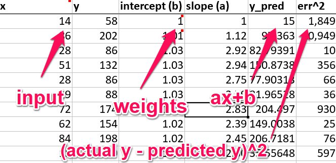 #
# Now, how do we improve our weights? Notice that the cost function (step 2 above) will be closer to 0 when the prediction is closer to the actual value. So we want to minimize this cost function. To minimize a function, we can:
#
# 1. Calculate the gradient of the function (the slope of steepest ascent)
# 2. Step "down" the gradient by some learning rate
#
# (I think there might be a slightly mistake in the Excel file here, as it assumes the cost function is predicted - actual, which flips a sign on the derivative, but it still works)
#
# So, we can write our cost (error) function as:
#
# $((ax+b)-y)^2$
#
# ($ax+b$ is our prediction, $y$ is our actual value).
#
# If we calculate the partial derivatives for this...
#
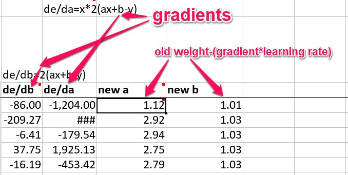
# The change in our function with respect to $b$ gives us:
#
# $\frac{\delta{e}}{\delta{b}} = 2(ax+b-y)$
#
# And with $a$:
#
# $\frac{\delta{e}}{\delta{a}} = 2x(ax+b-y)$
#
# So, to update our weights, we calulate the gradients using this formula, and then do:
#
# $new\_weight = old\_weight-(gradient*learning\_rate)$
#
# This gives us some weights that should decrease our cost function on the next iteration (at least they would for the sample we just ran), and so we repeat the cycle with them.
#
#
#
# Now, how do we improve our weights? Notice that the cost function (step 2 above) will be closer to 0 when the prediction is closer to the actual value. So we want to minimize this cost function. To minimize a function, we can:
#
# 1. Calculate the gradient of the function (the slope of steepest ascent)
# 2. Step "down" the gradient by some learning rate
#
# (I think there might be a slightly mistake in the Excel file here, as it assumes the cost function is predicted - actual, which flips a sign on the derivative, but it still works)
#
# So, we can write our cost (error) function as:
#
# $((ax+b)-y)^2$
#
# ($ax+b$ is our prediction, $y$ is our actual value).
#
# If we calculate the partial derivatives for this...
#
# The change in our function with respect to $b$ gives us:
#
# $\frac{\delta{e}}{\delta{b}} = 2(ax+b-y)$
#
# And with $a$:
#
# $\frac{\delta{e}}{\delta{a}} = 2x(ax+b-y)$
#
# So, to update our weights, we calulate the gradients using this formula, and then do:
#
# $new\_weight = old\_weight-(gradient*learning\_rate)$
#
# This gives us some weights that should decrease our cost function on the next iteration (at least they would for the sample we just ran), and so we repeat the cycle with them.
#
#  #
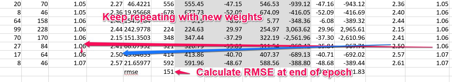
# Once we have ran through all of our data, we have completed one epoch of training, and we can calculate the RMSE for our entire data set, and start another epoch.
#
#
#
# Once we have ran through all of our data, we have completed one epoch of training, and we can calculate the RMSE for our entire data set, and start another epoch.
#
#  #
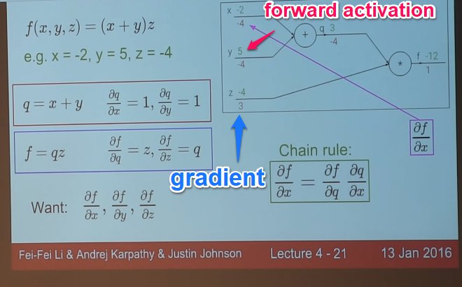
# ### Gradient Descent as Circuit/Chain Rule
#
# Ref: https://www.youtube.com/watch?v=i94OvYb6noo
#
# It's been suggested that backpropagation is just "keep applying the chain rule". This video has a good explanation and examples.
#
# During the forward pass, we also store the derivative of each of our function "gates", then, during the backprop, we multiply the previous gradient by the gradient for this gate, and so on. This lets us run backprop with around the same efficiency as the forward pass. It would be far too complex to try and compute a huge derivative for the entire function, so we do it bit by bit instead. In fact, if you look at PyTorch, a lot of it consists of these "gate" modules.
#
#
#
# ### Gradient Descent as Circuit/Chain Rule
#
# Ref: https://www.youtube.com/watch?v=i94OvYb6noo
#
# It's been suggested that backpropagation is just "keep applying the chain rule". This video has a good explanation and examples.
#
# During the forward pass, we also store the derivative of each of our function "gates", then, during the backprop, we multiply the previous gradient by the gradient for this gate, and so on. This lets us run backprop with around the same efficiency as the forward pass. It would be far too complex to try and compute a huge derivative for the entire function, so we do it bit by bit instead. In fact, if you look at PyTorch, a lot of it consists of these "gate" modules.
#
#  #
#
#
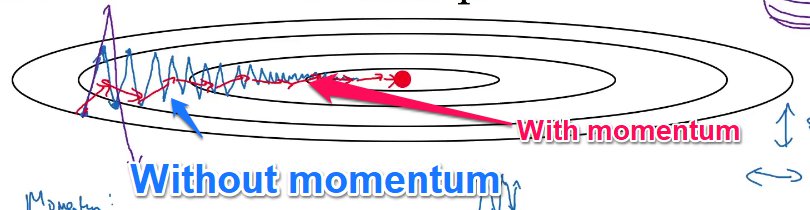
# ## Momentum
# One problem with gradient descent is that it is slow and tends to have problems in "ravines" (areas of a surface where one side if steeper than another). In this case, the function can tend to oscillate across the slopes.
#
# The intuition behind momentum is that it's like rolling a ball down a slope instead of walking down the slope. The inertia of the ball helps to speed up our descent and dampen oscillations.
#
#
#
#
#
# ## Momentum
# One problem with gradient descent is that it is slow and tends to have problems in "ravines" (areas of a surface where one side if steeper than another). In this case, the function can tend to oscillate across the slopes.
#
# The intuition behind momentum is that it's like rolling a ball down a slope instead of walking down the slope. The inertia of the ball helps to speed up our descent and dampen oscillations.
#
#  #
# Technical definition:
# _Use an exponentially weighted average of your gradients to update your weights_
#
# or from fast.ai:
#
# _Combines a decaying average of our previous gradients with the current gradient_
#
# You can think of it like averaging over the last $1/1-beta$ points in your sequence. So if beta was around 0.9, we're averaging over approximately the last 10 gradients.
#
# Momentum typically uses two hyperparameters:
#
# $\beta$ = some value between 0-1
#
# $\alpha$ = $1-\beta$
#
# Usually $\beta$ is set to 0.9, making $\alpha$ 0.1. Momentum will almost always result in faster learning than standard SGD.
#
# The momentum algorithm works like this ($v_\delta{w}$ is our new momentum gradient):
#
# 1. Calulate the gradient $\delta{W}$ like usual
# 2. Calculate our new "momentum" gradient: $v_\delta{w} = \beta v_\delta{w} + (1-\beta)\delta{W}$
# 3. Use this new gradient to update the weights: $W = W-{learning\_rate}*v_\delta{w}$
#
# It's like we are remembering our last gradient, and adding on just a bit of the new gradient. Hence the fast.ai definition above.
# ## RMSProp
# A gradient descent optimization method. Like momentum, it speeds up vertical descent while minimizing oscillations.
#
# Stands for __Root Mean Square prop__.
#
# Imagine we have two axes:
#
# * b: vertical axis
# * w: horizontal axis
#
# Then for each iteration:
#
# $S_{\delta{w}} = \beta{S_{\delta{w}}} + (1-\beta)\delta{w}^2$
# -- The new gradient is the old gradient * $\beta$ + $1-\beta$ * the gradient of w squared.
# Like momentum, this is keeping an exponentially weighted average but with the squares of the derivatives. You are storing the old square of the derivatives, and adding on a bit of the new one.
#
# $S_{\delta{b}} = \beta{S_{\delta{b}}} + (1-\beta)\delta{b}^2$
#
# Now, w gets updated as:
#
# $w = w-\alpha{\frac{\delta{w}}{\sqrt{S_{\delta{w}}}+ \epsilon}}$
#
# and
#
# $b = b-\alpha{\frac{\delta{b}}{\sqrt{S_{\delta{b}}}+ \epsilon}}$
#
# $(\alpha = learning\_rate)$
#
# To stop the math blowing up, we add $\epsilon$, which is typically a very small value like $10^{-8}$.
#
# If this is happening for every weight, then every weight effectively has a different learning rate.
#
# The idea is that $S_{\delta{w}}$ will be small, resulting in $w$ being larger -- accelerating horizontal movement, and $S_{\delta{b}}$ will be large, resulting in $b$ being smaller -- minimizing movement in the vertical direction.
#
# The name is derived because you are squaring the derivative, and then taking the square root in the division step.
# ## Adam
# Momentum + RMSProp. Stands for __Adaptive Moment Estimation__.
#
# 1. First, compute the momentum $v_\delta{w} = \beta_1 v_\delta{w} + (1-\beta_1)\delta{W}$ (we use $\beta_1$ to distingush this $\beta$ from the $\beta$ for RMSProp)
# 2. Calculate RMSProp $S_{\delta{w}} = \beta_2{S_{\delta{w}}} + (1-\beta_2)\delta{w}^2$
#
# Now $v_\delta{w}$ and $S_{\delta{w}}$ are initialized to 0 an it has been observed that they tend to be biased towards 0, especially when decay rates are small. So we implement some bias correction.
#
# 3. Compute the bias correction for V: $V^{corrected}_{\delta{w}} = \frac{V_\delta{w}}{(1-\beta_1^t)}$ where $t$ is the number of iterations
# 3. Compute the bias correction S: $S^{corrected}_{\delta{w}} = \frac{S_\delta{w}}{(1-\beta_2^t)}$ where $t$ is the number of iterations
# 4. Now, we finally update our weights: $w = w-\alpha{\frac{V^{corrected}_{\delta{w}}}{\sqrt{S^{corrected}_{\delta{w}}}+ \epsilon}}$
#
# Suggested hyperparameter values are:
#
# * $\beta_1 = 0.999$
# * $\beta_2 = 0.9$
# * $\epsilon = 10^{-8}$
#
# $v_\delta{w}$ is estimating the mean of the derivatives. This is called the first moment.
#
# $S_{\delta{w}}$ is estimating the exponentially weighted average of the squares. This is called the second moment.
#
# Hence the name, _adaptive moment estimation_.
# ## Weight Decay/L2 Regulartization
# Overfitting is characterized by large weight values. The purpose of weight decay is to reduce the magnitude of weights, and thus reduce overfitting.
#
# When training our neural network, we come up with some error/cost. L2 regularization adds a factor to the error. This factor is a fraction of the sum of the squared weights. So larger weights will create a larger error, and smaller weights will be rewarded.
#
# When updating our weights normally, we use:
#
# $w' = w-\eta{\frac{\delta{C}}{\delta{w}}}$
#
# (New weight is the old weight - learning rate ($\eta$) * gradient.)
#
# When updating our weights with L2 regularization, we use:
#
# $w' = (1-\frac{\eta*\lambda}{n})w-\eta{\frac{\delta{C}}{\delta{w}}}$
#
# Where $n=$number of samples and $\lambda=$L2 regularization constant.
#
# In other words, before subtracting the gradient, we reduce the weight by 1 - learning rate * decay constant/number of samples. This causes the weights to tend to "decay" over time.
#
# In terms of practical implementation, the weights may be calculated as normal, and then a fraction of the original weight value subtracted after.
#
#
# In[ ]:
#
# Technical definition:
# _Use an exponentially weighted average of your gradients to update your weights_
#
# or from fast.ai:
#
# _Combines a decaying average of our previous gradients with the current gradient_
#
# You can think of it like averaging over the last $1/1-beta$ points in your sequence. So if beta was around 0.9, we're averaging over approximately the last 10 gradients.
#
# Momentum typically uses two hyperparameters:
#
# $\beta$ = some value between 0-1
#
# $\alpha$ = $1-\beta$
#
# Usually $\beta$ is set to 0.9, making $\alpha$ 0.1. Momentum will almost always result in faster learning than standard SGD.
#
# The momentum algorithm works like this ($v_\delta{w}$ is our new momentum gradient):
#
# 1. Calulate the gradient $\delta{W}$ like usual
# 2. Calculate our new "momentum" gradient: $v_\delta{w} = \beta v_\delta{w} + (1-\beta)\delta{W}$
# 3. Use this new gradient to update the weights: $W = W-{learning\_rate}*v_\delta{w}$
#
# It's like we are remembering our last gradient, and adding on just a bit of the new gradient. Hence the fast.ai definition above.
# ## RMSProp
# A gradient descent optimization method. Like momentum, it speeds up vertical descent while minimizing oscillations.
#
# Stands for __Root Mean Square prop__.
#
# Imagine we have two axes:
#
# * b: vertical axis
# * w: horizontal axis
#
# Then for each iteration:
#
# $S_{\delta{w}} = \beta{S_{\delta{w}}} + (1-\beta)\delta{w}^2$
# -- The new gradient is the old gradient * $\beta$ + $1-\beta$ * the gradient of w squared.
# Like momentum, this is keeping an exponentially weighted average but with the squares of the derivatives. You are storing the old square of the derivatives, and adding on a bit of the new one.
#
# $S_{\delta{b}} = \beta{S_{\delta{b}}} + (1-\beta)\delta{b}^2$
#
# Now, w gets updated as:
#
# $w = w-\alpha{\frac{\delta{w}}{\sqrt{S_{\delta{w}}}+ \epsilon}}$
#
# and
#
# $b = b-\alpha{\frac{\delta{b}}{\sqrt{S_{\delta{b}}}+ \epsilon}}$
#
# $(\alpha = learning\_rate)$
#
# To stop the math blowing up, we add $\epsilon$, which is typically a very small value like $10^{-8}$.
#
# If this is happening for every weight, then every weight effectively has a different learning rate.
#
# The idea is that $S_{\delta{w}}$ will be small, resulting in $w$ being larger -- accelerating horizontal movement, and $S_{\delta{b}}$ will be large, resulting in $b$ being smaller -- minimizing movement in the vertical direction.
#
# The name is derived because you are squaring the derivative, and then taking the square root in the division step.
# ## Adam
# Momentum + RMSProp. Stands for __Adaptive Moment Estimation__.
#
# 1. First, compute the momentum $v_\delta{w} = \beta_1 v_\delta{w} + (1-\beta_1)\delta{W}$ (we use $\beta_1$ to distingush this $\beta$ from the $\beta$ for RMSProp)
# 2. Calculate RMSProp $S_{\delta{w}} = \beta_2{S_{\delta{w}}} + (1-\beta_2)\delta{w}^2$
#
# Now $v_\delta{w}$ and $S_{\delta{w}}$ are initialized to 0 an it has been observed that they tend to be biased towards 0, especially when decay rates are small. So we implement some bias correction.
#
# 3. Compute the bias correction for V: $V^{corrected}_{\delta{w}} = \frac{V_\delta{w}}{(1-\beta_1^t)}$ where $t$ is the number of iterations
# 3. Compute the bias correction S: $S^{corrected}_{\delta{w}} = \frac{S_\delta{w}}{(1-\beta_2^t)}$ where $t$ is the number of iterations
# 4. Now, we finally update our weights: $w = w-\alpha{\frac{V^{corrected}_{\delta{w}}}{\sqrt{S^{corrected}_{\delta{w}}}+ \epsilon}}$
#
# Suggested hyperparameter values are:
#
# * $\beta_1 = 0.999$
# * $\beta_2 = 0.9$
# * $\epsilon = 10^{-8}$
#
# $v_\delta{w}$ is estimating the mean of the derivatives. This is called the first moment.
#
# $S_{\delta{w}}$ is estimating the exponentially weighted average of the squares. This is called the second moment.
#
# Hence the name, _adaptive moment estimation_.
# ## Weight Decay/L2 Regulartization
# Overfitting is characterized by large weight values. The purpose of weight decay is to reduce the magnitude of weights, and thus reduce overfitting.
#
# When training our neural network, we come up with some error/cost. L2 regularization adds a factor to the error. This factor is a fraction of the sum of the squared weights. So larger weights will create a larger error, and smaller weights will be rewarded.
#
# When updating our weights normally, we use:
#
# $w' = w-\eta{\frac{\delta{C}}{\delta{w}}}$
#
# (New weight is the old weight - learning rate ($\eta$) * gradient.)
#
# When updating our weights with L2 regularization, we use:
#
# $w' = (1-\frac{\eta*\lambda}{n})w-\eta{\frac{\delta{C}}{\delta{w}}}$
#
# Where $n=$number of samples and $\lambda=$L2 regularization constant.
#
# In other words, before subtracting the gradient, we reduce the weight by 1 - learning rate * decay constant/number of samples. This causes the weights to tend to "decay" over time.
#
# In terms of practical implementation, the weights may be calculated as normal, and then a fraction of the original weight value subtracted after.
#
#
# In[ ]: