#!/usr/bin/env python
# coding: utf-8

# # Lecture 17:  Tensor decompositions

# ## Recap of the previous lecture
# * Wavelets
# * L1-norm minimization
# * Compressed sensing

# ## Today lecture 
# 
# * Tensor decompositions and applications
# * Practice

# # Tensors
# 
# By **tensor** we imply nothing, but a **multidimensional array**:
# $$
# A(i_1, \dots, i_d), \quad 1\leq i_k\leq n_k,
# $$
# where $d$ is called dimension, $n_k$ - mode size.
# This is standard definition in applied mathematics community. For details see [[1]](http://citeseerx.ist.psu.edu/viewdoc/download?doi=10.1.1.153.2059&rep=rep1&type=pdf), [[2]](http://arxiv.org/pdf/1302.7121.pdf), [[3]](http://epubs.siam.org/doi/abs/10.1137/090752286).
# 
# * $d=2$ (matrices) $\Rightarrow$ classic theory (SVD, LU, QR, $\dots$)
# 
# * $d\geq 3$ (tensors) $\Rightarrow$ under development. Generalization of standard matrix results is not always straightforward

# ## Curse of dimensionality
# 
# The problem with multidimensional data is that number of parameters grows <font color='red'> exponentially </font> with $d$:
# 
# 
# $$
#     \text{storage} = n^d.
# $$
# For instance, for $n=2$ and $d=500$
# $$
#     n^d = 2^{500} \gg 10^{83}  -  \text{ number of atoms in the Universe}
# $$
# 
# Why do we care? It seems that we are living in the 3D World :)

# ## Applications
# 
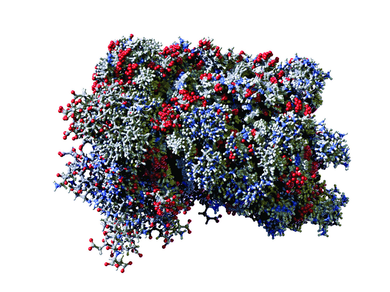
# #### Quantum chemistry
# 
# Stationary Schroedinger equation for system with $N_{el}$ electrons
# $$
#     \hat H \Psi = E \Psi,
# $$
# where
# $$
# \Psi = \Psi(\{{\bf r_1},\sigma_1\},\dots, \{{\bf r_{N_{el}}},\sigma_{N_{el}}\})
# $$
# 3$N_{el}$ spatial variables and $N_{el}$ spin variable. 
# <img src="http://blog.covance.com/wp-content/uploads/2015/02/101679_Large-Molecule_1575263331.jpg" width=400>
# 
# * Drug and material design
# * Predicting physical experiments

# #### Uncertainty quantification
# 
# Example: oil reservoir modeling. Model may depend on parameters $p_1,\dots,p_d$ (like measured experimentally procity or temperature) with uncertainty
# 
# $$
# u = u(t,{\bf r},\,{p_1,\dots,p_d})
# $$
# <img src='http://www.ife.no/en/ife/departments/tracer/tracertechnology/image' width=350>

# #### And many more
# 
# * Signal processing
# * Recommender systems
# * Neural networks
# * Language models
# * Financial mathematics
# * ...

# ## Working with many dimensions
# 
# * **Monte-Carlo**: class of methods based on random sampling. Convergence issues
# * **Sparse grids**: special types of grids with small number of grid points. Strong regularity conditions
# * Young and promising approach based on <font color='red'>tensor decompositions </font>

# ## Tensor decompositions
# 
# ## 2D
# 
# Skeleton decomposition:
# $$
# A = UV^T
# $$
# or elementwise:
# $$
# a_{ij} = \sum_{\alpha=1}^r u_{i\alpha} v_{j\alpha}
# $$
# leads us to the idea of **separation of variables.**
# 
# **Properties:**
# * Not unique: $A = U V^T = UBB^{-1}V^T = \tilde U \tilde V^T$
# * Can be calculated in a stable way by **SVD**

# ## 1. Canonical decomposition
# 
# The most straightforward way to generize separation of variables to many dimensions is the **canonical decomposition**: (CP/CANDECOMP/PARAFAC)
# $$
# a_{ijk} = \sum_{\alpha=1}^r u_{i\alpha} v_{j\alpha} w_{k\alpha}
# $$
# minimal possible $r$ is called the **canonical rank**. Matrices $U$, $V$ and $W$ are called **canonical factors**. This decomposition was proposed in 1927 by Hitchcock.

# **Properties**:
# 
# * For a $d$ dimensional tensor memory is $nrd$
# * Unique under mild conditions
# * Set of tensors with rank$\leq r$ is not closed (by contrast to matrices): <br>
#   $a_{ijk} = i+j+k$, $\text{rank}(A) = 3$, but
#   $$
#       a^\epsilon_{ijk} = \frac{(1+\epsilon i)(1+\epsilon j)(1+\epsilon k) - 1}{\epsilon}\to i+j+k=a_{ijk},\quad \epsilon\to 0
#   $$
#   and $\text{rank}(A^{\epsilon}) = 2$
# * No stable algorithms to compute best rank-$r$ approximation

# **Alternating Least Squares algorithm**
# 
# 0. Intialize random $U,V,W$
# 1. fix $V,W$, solve least squares for $U$
# 2. fix $U,W$, solve least squares for $V$
# 3. fix $U,V$, solve least squares for $W$
# 4. go to 2.

# ## 2. Tucker decomposition
# 
# Next attempt is the decomposition proposed by Tucker in 1963 in chemometrics journal:
# $$
# a_{ijk} = \sum_{\alpha_1,\alpha_2,\alpha_3=1}^{r_1,r_2,r_3}g_{\alpha_1\alpha_2\alpha_3} u_{i\alpha_1} v_{j\alpha_2} w_{k\alpha_3}.
# $$
# Here we have several different ranks. Minimal possible $r_1,r_2,r_3$ are called **Tucker ranks**.
# 
# **Properties**:
# 
# * For a $d$ dimensional tensor memory is <font color='red'>$r^d$</font> $+ nrd$. Still **curse of dimensionality**
# * Stable SVD-based algorithm:
#     1. $U =$ principal components of the unfolding `A.reshape(n1, n2*n3)`
#     2. $V =$ principal components of the unfolding `A.transpose([1,0,2]).reshape(n2, n1*n3)`
#     3. $W =$ principal components of the unfolding `A.transpose([2,0,1]).reshape(n3, n1*n2)`
#     4. $g_{\alpha_1\alpha_2\alpha_3} = \sum_{i,j,k=1}^{n_1,n_2,n_3} a_{ijk} u_{i\alpha_1} v_{j\alpha_2} w_{k\alpha_3}$.

# ## 3. Tensor Train decomposition
# 
# * Calculation of the canonical decomposition is unstable
# * Tucker decomposition suffers from the curse of dimensionality
# 
# Tensor Train (**TT**) decomposition (Oseledets, Tyrtyshnikov 2009) is both stable and contains linear in $d$ number of parameters:
# $$
# a_{i_1 i_2 \dots i_d} = \sum_{\alpha_1,\dots,\alpha_{d-1}} 
# g_{i_1\alpha_1} g_{\alpha_1 i_2\alpha_2}\dots g_{\alpha_{d-2} i_{d-1}\alpha_{d-1}} g_{\alpha_{d-1} i_{d}}
# $$
# or in the matrix form
# $$
#     a_{i_1 i_2 \dots i_d} = G_1 (i_1)G_2 (i_2)\dots G_d(i_d)
# $$
# * The storage is $\mathcal{O}(dnr^2)$ 
# * Stable TT-SVD algorithm

# **Example**
# $$a_{i_1\dots i_d} = i_1 + \dots + i_d$$
# Canonical rank is $d$. At the same time TT-ranks are $2$:
# $$
# i_1 + \dots + i_d = \begin{pmatrix} i_1 & 1 \end{pmatrix} 
# \begin{pmatrix} 1 & 0 \\ i_2 & 1 \end{pmatrix}
# \dots
# \begin{pmatrix} 1 & 0 \\ i_{d-1} & 1 \end{pmatrix}
# \begin{pmatrix} 1  \\  i_d \end{pmatrix}
# $$

# ## 4. Quantized Tensor Train
# 
# Consider a 1D array $a_k = f(x_k)$, $k=1,\dots,2^d$ where $f$ is some 1D function calculated on grid points $x_k$.
# 
# Let $$k = {2^{d-1} i_1 + 2^{d-2} i_2 + \dots + 2^0 i_{d}}\quad i_1,\dots,i_d = 0,1 $$ 
# be binary representation of $k$, then
# $$
#     a_k = a_{2^{d-1} i_1 + 2^{d-2} i_2 + \dots + 2^0 i_{d}} \equiv \tilde a_{i_1,\dots,i_d},
# $$
# where $\tilde a$ is nothing, but a reshaped tensor $a$. TT decomposition of $\tilde a$ is called **Quantized Tensor Train (QTT)** decomposition. Interesting fact is that the QTT decomposition has relation to wavelets.
# 
# Contains <font color='red'>$\mathcal{O}(\log n r^2)$</font> elements!

# ## Cross approximation method
# 
# If decomposition of a tensor is given, then there is no problem to do basic operations fast. 
# 
# However, the question is if it is possible to find decomposition taking into account that typically tensors even can not be stored. 
# 
# **Cross approximation** method allows to find the decomposition using only few of its elements.

# ## Summary 
# 
# * Tensor decompositions - useful tool to work with multidimensional data
# * Canonical, Tucker, TT, QTT decompositions
# * Cross approximation

# ## Next time
# 
# Ping-Pong test

# ## Now lets have some practice

# In[1]:


from IPython.core.display import HTML
def css_styling():
    styles = open("./styles/custom.css", "r").read()
    return HTML(styles)
css_styling()