# ![]() #
#
#
#
IRIS-EarthScope Short Course
#Bloomington/IN, August 2015
##
Python/ObsPy Introduction
## #
# ![]() #
#
#
#
 #
# * the "[`get_events()`](https://docs.obspy.org/packages/autogen/obspy.fdsn.client.Client.get_events.html)" method has many ways to restrict the search results (time, geographic, magnitude, ..)
# In[ ]:
from obspy.fdsn import Client
client = Client("IRIS")
catalog = client.get_events(minmagnitude=8.5, starttime="2010-01-01")
print(catalog)
catalog.plot();
# - event/earthquake metadata is bundled in a **`Catalog`** object, which is a collection (~list) of **`Event`** objects
# - `Event` objects are again collections of other resources (origins, magnitudes, picks, ...)
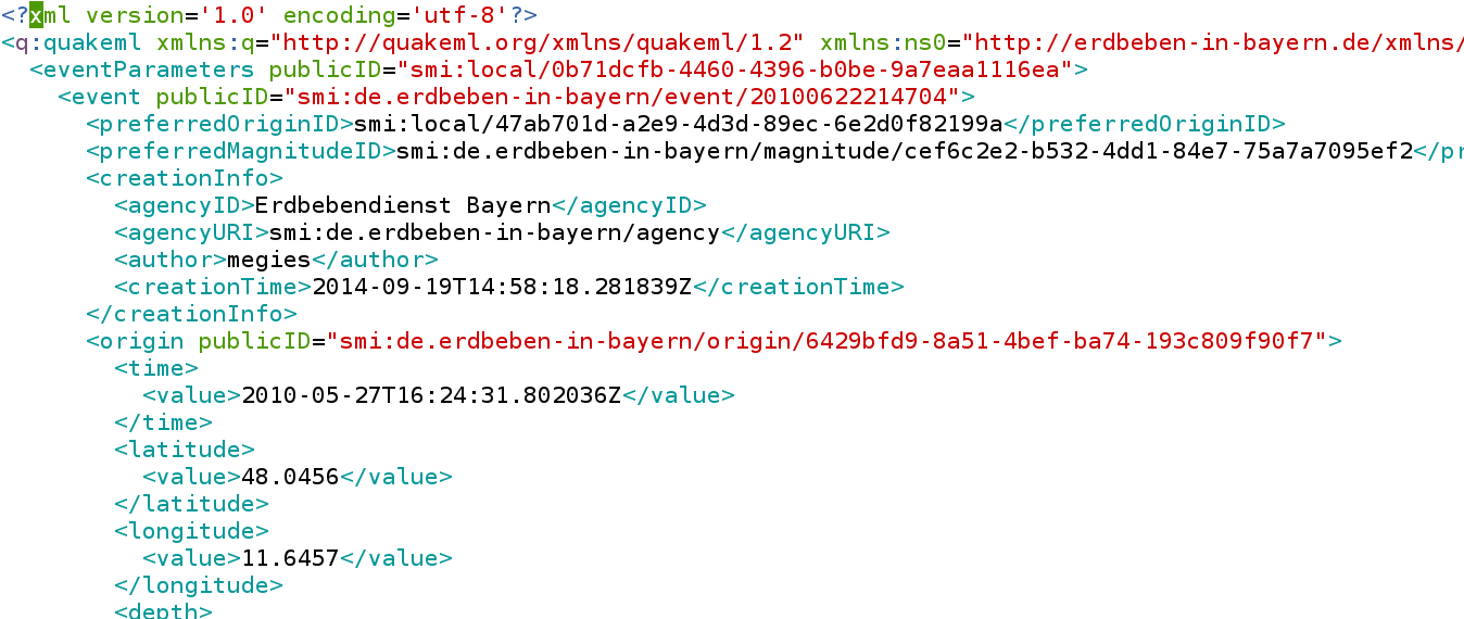
# - the nested ObsPy Event class structure (Catalog/Event/Origin/Magnitude/FocalMechanism/...) is closely modelled after [QuakeML](https://quake.ethz.ch/quakeml) (the international standard exchange format for event metadata)
#
#
# * the "[`get_events()`](https://docs.obspy.org/packages/autogen/obspy.fdsn.client.Client.get_events.html)" method has many ways to restrict the search results (time, geographic, magnitude, ..)
# In[ ]:
from obspy.fdsn import Client
client = Client("IRIS")
catalog = client.get_events(minmagnitude=8.5, starttime="2010-01-01")
print(catalog)
catalog.plot();
# - event/earthquake metadata is bundled in a **`Catalog`** object, which is a collection (~list) of **`Event`** objects
# - `Event` objects are again collections of other resources (origins, magnitudes, picks, ...)
# - the nested ObsPy Event class structure (Catalog/Event/Origin/Magnitude/FocalMechanism/...) is closely modelled after [QuakeML](https://quake.ethz.ch/quakeml) (the international standard exchange format for event metadata)
#  #
#  # In[ ]:
print(catalog)
# In[ ]:
event = catalog[1]
print(event)
# In[ ]:
# you can use Tab-Completion to see what attributes/methods the event object has:
event.
origin.
# * local files can be read using the [`readEvents()`](https://docs.obspy.org/packages/autogen/obspy.core.event.readEvents.html) function.
# In[ ]:
from obspy import readEvents
catalog2 = readEvents("./data/events_unterhaching.xml")
print(catalog2)
# these events contain picks, too
print(catalog2[0].picks[0])
# ### 2. Station Metadata
#
# * again, several different protocols are implemented in ObsPy to connect to all important seismological data centers
# * the most important protocol are [FDSN web services](https://docs.obspy.org/packages/obspy.fdsn.html) (other protocols work similar)
# * the "[`get_stations()`](https://docs.obspy.org/packages/autogen/obspy.fdsn.client.Client.get_stations.html)" method has many ways to restrict the search results (time, geographic, station names, ..)
# In[ ]:
t = event.origins[0].time
print(t)
inventory = client.get_stations(
network="TA",
starttime=t, endtime=t+10)
print(inventory)
inventory.plot(projection="local");
# - station metadata is bundled in an **`Inventory`** object, which is a collection (~list) of **`Network`** objects, ...
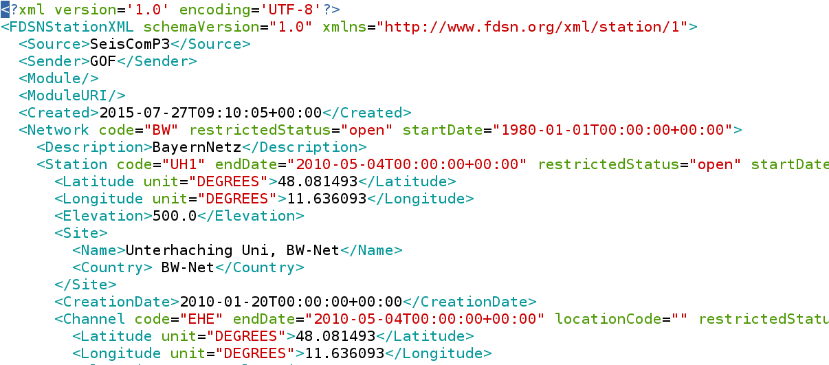
# - the nested ObsPy Inventory class structure (Inventory/Network/Station/Channel/Response/...) is closely modelled after [FDSN StationXML](https://www.fdsn.org/xml/station/) (the international standard exchange format for station metadata)
# - `Network` objects are again collections of `Station` objects, which are collections of `Channel` objects
#
#
# In[ ]:
print(catalog)
# In[ ]:
event = catalog[1]
print(event)
# In[ ]:
# you can use Tab-Completion to see what attributes/methods the event object has:
event.
origin.
# * local files can be read using the [`readEvents()`](https://docs.obspy.org/packages/autogen/obspy.core.event.readEvents.html) function.
# In[ ]:
from obspy import readEvents
catalog2 = readEvents("./data/events_unterhaching.xml")
print(catalog2)
# these events contain picks, too
print(catalog2[0].picks[0])
# ### 2. Station Metadata
#
# * again, several different protocols are implemented in ObsPy to connect to all important seismological data centers
# * the most important protocol are [FDSN web services](https://docs.obspy.org/packages/obspy.fdsn.html) (other protocols work similar)
# * the "[`get_stations()`](https://docs.obspy.org/packages/autogen/obspy.fdsn.client.Client.get_stations.html)" method has many ways to restrict the search results (time, geographic, station names, ..)
# In[ ]:
t = event.origins[0].time
print(t)
inventory = client.get_stations(
network="TA",
starttime=t, endtime=t+10)
print(inventory)
inventory.plot(projection="local");
# - station metadata is bundled in an **`Inventory`** object, which is a collection (~list) of **`Network`** objects, ...
# - the nested ObsPy Inventory class structure (Inventory/Network/Station/Channel/Response/...) is closely modelled after [FDSN StationXML](https://www.fdsn.org/xml/station/) (the international standard exchange format for station metadata)
# - `Network` objects are again collections of `Station` objects, which are collections of `Channel` objects
#
#  #
#  # In[ ]:
# let's request full detail metadata for one particular station
inventory = client.get_stations(network="TA", station="S36A", level="response")
# when searching for many available stations response information is not included by default,
# because of the huge size. we explicitly need to specify that we want response information included
print(inventory)
# In[ ]:
network = inventory[0]
print(network)
# In[ ]:
station = network[0]
print(station)
# In[ ]:
station = station.select(channel="BH*")
print(station)
# In[ ]:
channel = station[0]
print(channel)
print(channel.response)
# In[ ]:
# you can use Tab-Completion to see what attributes/methods the inventory object has:
inventory.
channel.
# * local files can be read using the [`read_inventory()`](https://docs.obspy.org/packages/autogen/obspy.station.inventory.read_inventory.html) function.
# * filetype is autodetected (but many real-world StationXML files do not adhere to the official schema, explicitly specify `format="STATIONXML"` in that case!)
# In[ ]:
from obspy import read_inventory
inventory2 = read_inventory("./data/station_uh1.xml", format="STATIONXML")
print(inventory2)
# ### 3. Waveform Data (seismometer time series)
#
# * again, several different protocols are implemented in ObsPy to connect to all important seismological data centers
# * also, local files in all important exchange formats can be read
# * the most important protocol are [FDSN web services](https://docs.obspy.org/packages/obspy.fdsn.html) (other protocols work similar)
# * real time data can be accessed using [`obspy.seedlink`](https://docs.obspy.org/packages/obspy.seedlink.html)
# * the "[`get_waveforms()`](https://docs.obspy.org/packages/autogen/obspy.fdsn.client.Client.get_waveforms.html)" method needs the unique identification of the station (network, station, location and channel codes) and a time range (start time, end time) of requested data
# In[ ]:
stream = client.get_waveforms(network="TA", station="S36A",
location="*", channel="BH*",
starttime=t+10*60, endtime=t+70*60)
# for functions/methods that need a fixed set of parameters,
# we usually omit the parameter names and specify them in the expected order
# Note that new timestamp objects can be created by
# adding/subtracting seconds to/from an existing timestamp object.
# (for details search the ObsPy documentation pages for "UTCDateTime")
stream = client.get_waveforms("TA", "S36A", "*", "BH*", t+10*60, t+70*60)
print(stream)
stream.plot()
# the nested ObsPy Inventory class structure (Inventory/Station/Channel/Response/...) is closely modelled after [FDSN StationXML](https://www.fdsn.org/xml/station/) (the international standard exchange format for station metadata)
#
# - waveform data is bundled in a **`Stream`** object, which is a collection (~list) of **`Trace`** objects
# - **`Trace`** objects consist of one single, contiguous waveform data block (i.e. regularly spaced time series, no gaps)
# - **`Trace`** objects consist of two attributes:
# - **`trace.data`** (the raw time series as an [**`numpy.ndarray`**](https://docs.scipy.org/doc/numpy/reference/generated/numpy.ndarray.html)) and..
# - **`trace.stats`** (metainformation needed to interpret the raw sample data)
#
#
# In[ ]:
# let's request full detail metadata for one particular station
inventory = client.get_stations(network="TA", station="S36A", level="response")
# when searching for many available stations response information is not included by default,
# because of the huge size. we explicitly need to specify that we want response information included
print(inventory)
# In[ ]:
network = inventory[0]
print(network)
# In[ ]:
station = network[0]
print(station)
# In[ ]:
station = station.select(channel="BH*")
print(station)
# In[ ]:
channel = station[0]
print(channel)
print(channel.response)
# In[ ]:
# you can use Tab-Completion to see what attributes/methods the inventory object has:
inventory.
channel.
# * local files can be read using the [`read_inventory()`](https://docs.obspy.org/packages/autogen/obspy.station.inventory.read_inventory.html) function.
# * filetype is autodetected (but many real-world StationXML files do not adhere to the official schema, explicitly specify `format="STATIONXML"` in that case!)
# In[ ]:
from obspy import read_inventory
inventory2 = read_inventory("./data/station_uh1.xml", format="STATIONXML")
print(inventory2)
# ### 3. Waveform Data (seismometer time series)
#
# * again, several different protocols are implemented in ObsPy to connect to all important seismological data centers
# * also, local files in all important exchange formats can be read
# * the most important protocol are [FDSN web services](https://docs.obspy.org/packages/obspy.fdsn.html) (other protocols work similar)
# * real time data can be accessed using [`obspy.seedlink`](https://docs.obspy.org/packages/obspy.seedlink.html)
# * the "[`get_waveforms()`](https://docs.obspy.org/packages/autogen/obspy.fdsn.client.Client.get_waveforms.html)" method needs the unique identification of the station (network, station, location and channel codes) and a time range (start time, end time) of requested data
# In[ ]:
stream = client.get_waveforms(network="TA", station="S36A",
location="*", channel="BH*",
starttime=t+10*60, endtime=t+70*60)
# for functions/methods that need a fixed set of parameters,
# we usually omit the parameter names and specify them in the expected order
# Note that new timestamp objects can be created by
# adding/subtracting seconds to/from an existing timestamp object.
# (for details search the ObsPy documentation pages for "UTCDateTime")
stream = client.get_waveforms("TA", "S36A", "*", "BH*", t+10*60, t+70*60)
print(stream)
stream.plot()
# the nested ObsPy Inventory class structure (Inventory/Station/Channel/Response/...) is closely modelled after [FDSN StationXML](https://www.fdsn.org/xml/station/) (the international standard exchange format for station metadata)
#
# - waveform data is bundled in a **`Stream`** object, which is a collection (~list) of **`Trace`** objects
# - **`Trace`** objects consist of one single, contiguous waveform data block (i.e. regularly spaced time series, no gaps)
# - **`Trace`** objects consist of two attributes:
# - **`trace.data`** (the raw time series as an [**`numpy.ndarray`**](https://docs.scipy.org/doc/numpy/reference/generated/numpy.ndarray.html)) and..
# - **`trace.stats`** (metainformation needed to interpret the raw sample data)
#
#  # In[ ]:
trace = stream[0]
# trace.data is the numpy array with the raw samples
print(trace.data)
print(trace.data[20:30])
# arithmetic operations on the data
print(trace.data[20:30] / 223.5)
# using attached numpy methods
print(trace.data.mean())
# pointers to the array in memory can be passed to C/Fortran routines from inside Python!
# In[ ]:
# trace.stats contains the basic metadata identifying the trace
print(trace)
print(trace.stats)
print(trace.stats.sampling_rate)
# In[ ]:
# many convenience routines are attahed to Stream/Trace, use Tab completion
stream.
# * local files can be read using the [`read()`](https://docs.obspy.org/packages/autogen/obspy.core.stream.read.html) function.
# * filetype is autodetected (but can be manually specified to skip autodetection for speed)
# In[ ]:
from obspy import read
stream2 = read("./data/waveforms_uh1_eh?.mseed")
print(stream2)
# * timestamps are handled by [`UTCDateTime`](https://docs.obspy.org/packages/autogen/obspy.core.utcdatetime.UTCDateTime.html) class throughout ObsPy
# In[ ]:
from obspy import UTCDateTime
t1 = UTCDateTime("2015-08-04T10:30")
print(t1.hour)
print(t1.strftime("%c"))
# * `+/-` operator to add/subtract seconds
# * `-` operator to get diff of two timestamps in seconds
# In[ ]:
# calculate time since Tohoku earthquake in years
now = UTCDateTime()
print((now - t) / (3600 * 24 * 365))
# 2 hours from now
print(now + 2 * 3600)
# ### 4. Converting raw seismometer recordings to physical units (aka instrument correction)
#
# * for this we need to combine the raw waveform data of the recording system (seismometer, digitizer) with the metadata on its amplitude and phase response (the instrument response)
# * these information are kept separate for various practical and technical reasons (space in storage and streaming, correcting of errors made in the metadata, ...)
# In[ ]:
# first, let's have a look at this channel's instrument response
channel.plot(min_freq=1e-4);
# In[ ]:
# we already have fetched the station metadata,
# including every piece of information down to the instrument response
# let's make on a copy of the raw data, to be able to compare afterwards
stream_corrected = stream.copy()
# attach the instrument response to the waveforms..
stream_corrected.attach_response(inventory)
# and convert the data to ground velocity in m/s,
# taking into account the specifics of the recording system
stream_corrected.remove_response(water_level=10, output="VEL")
stream[0].plot()
stream_corrected[0].plot()
# ### ObsPy has much more functionality, check it out on the ObsPy documentation pages at https://docs.obspy.org.
#
# * many, many convenience routines attached to `Stream`/`Trace`, `Catalog`/`Event`/.., `Inventory`/... for easy manipulation
# * filtering, detrending, demeaning, rotating, resampling, ...
# * array analysis, cross correlation routines, event detection, ...
# * estimate travel times and [plot ray paths](https://docs.obspy.org/tutorial/code_snippets/travel_time.html#body-wave-ray-paths) of seismic phases for specified source/receiver combinations
# * command line utilities (`obspy-print`, `obspy-plot`, `obspy-scan`, ...)
# * ...
#
#
# In[ ]:
trace = stream[0]
# trace.data is the numpy array with the raw samples
print(trace.data)
print(trace.data[20:30])
# arithmetic operations on the data
print(trace.data[20:30] / 223.5)
# using attached numpy methods
print(trace.data.mean())
# pointers to the array in memory can be passed to C/Fortran routines from inside Python!
# In[ ]:
# trace.stats contains the basic metadata identifying the trace
print(trace)
print(trace.stats)
print(trace.stats.sampling_rate)
# In[ ]:
# many convenience routines are attahed to Stream/Trace, use Tab completion
stream.
# * local files can be read using the [`read()`](https://docs.obspy.org/packages/autogen/obspy.core.stream.read.html) function.
# * filetype is autodetected (but can be manually specified to skip autodetection for speed)
# In[ ]:
from obspy import read
stream2 = read("./data/waveforms_uh1_eh?.mseed")
print(stream2)
# * timestamps are handled by [`UTCDateTime`](https://docs.obspy.org/packages/autogen/obspy.core.utcdatetime.UTCDateTime.html) class throughout ObsPy
# In[ ]:
from obspy import UTCDateTime
t1 = UTCDateTime("2015-08-04T10:30")
print(t1.hour)
print(t1.strftime("%c"))
# * `+/-` operator to add/subtract seconds
# * `-` operator to get diff of two timestamps in seconds
# In[ ]:
# calculate time since Tohoku earthquake in years
now = UTCDateTime()
print((now - t) / (3600 * 24 * 365))
# 2 hours from now
print(now + 2 * 3600)
# ### 4. Converting raw seismometer recordings to physical units (aka instrument correction)
#
# * for this we need to combine the raw waveform data of the recording system (seismometer, digitizer) with the metadata on its amplitude and phase response (the instrument response)
# * these information are kept separate for various practical and technical reasons (space in storage and streaming, correcting of errors made in the metadata, ...)
# In[ ]:
# first, let's have a look at this channel's instrument response
channel.plot(min_freq=1e-4);
# In[ ]:
# we already have fetched the station metadata,
# including every piece of information down to the instrument response
# let's make on a copy of the raw data, to be able to compare afterwards
stream_corrected = stream.copy()
# attach the instrument response to the waveforms..
stream_corrected.attach_response(inventory)
# and convert the data to ground velocity in m/s,
# taking into account the specifics of the recording system
stream_corrected.remove_response(water_level=10, output="VEL")
stream[0].plot()
stream_corrected[0].plot()
# ### ObsPy has much more functionality, check it out on the ObsPy documentation pages at https://docs.obspy.org.
#
# * many, many convenience routines attached to `Stream`/`Trace`, `Catalog`/`Event`/.., `Inventory`/... for easy manipulation
# * filtering, detrending, demeaning, rotating, resampling, ...
# * array analysis, cross correlation routines, event detection, ...
# * estimate travel times and [plot ray paths](https://docs.obspy.org/tutorial/code_snippets/travel_time.html#body-wave-ray-paths) of seismic phases for specified source/receiver combinations
# * command line utilities (`obspy-print`, `obspy-plot`, `obspy-scan`, ...)
# * ...
#
#  #
# ---
# ### Automated Data Fetching/Processing Example
#
# This example prepares instrument corrected waveforms, 30 seconds around expected P arrival (buffer for processing!) for an epicentral range of 30-40 degrees for any TA station/earthquake combination with magnitude larger 7.
# In[ ]:
from obspy.taup import TauPyModel
from obspy.core.util.geodetics import gps2DistAzimuth, kilometer2degrees
model = TauPyModel(model="iasp91")
catalog = client.get_events(starttime="2009-001", endtime="2012-001", minmagnitude=7)
print(catalog)
network = "TA"
minradius = 30
maxradius = 40
phase = "P"
for event in catalog:
origin = event.origins[0]
try:
inventory = client.get_stations(network=network,
startbefore=origin.time, endafter=origin.time,
longitude=origin.longitude, latitude=origin.latitude,
minradius=minradius, maxradius=maxradius)
except:
continue
print(event)
for station in inventory[0][:3]:
distance, _, _ = gps2DistAzimuth(origin.latitude, origin.longitude,
station.latitude, station.longitude)
distance = kilometer2degrees(distance / 1e3)
arrivals = model.get_travel_times(origin.depth / 1e3, distance,
phase_list=[phase])
traveltime = arrivals[0].time
arrival_time = origin.time + traveltime
st = client.get_waveforms(network, station.code, "*", "BH*",
arrival_time - 200, arrival_time + 200,
attach_response=True)
st.remove_response(water_level=10, output="VEL")
st.filter("lowpass", freq=1)
st.trim(arrival_time - 10, arrival_time + 20)
st.plot()
break
# ## Exercise
#
# Problems? Questions?
#
# - [ObsPy Documentation](https://docs.obspy.org/) (use the search)
# - Use IPython tab completion
# - Use interactive IPython help (e.g. after import type: `readEvents?`)
# - **Ask!**
#
# a) Read the event metadata from local file "`./data/events_unterhaching.xml`". Print the catalog summary.
# In[ ]:
# b) Take one event out of the catalog. Print its summary. You can see, there is information included on picks set for the event. Print the information of at least one pick that is included in the event metadata. We now know one station that recorded the event.
# In[ ]:
# c) Save the origin time of the event in a new variable. Download waveform data for the station around the time of the event (e.g. 10 seconds before and 20 seconds after), connecting to the FDSN server at the observatory at "`http://erde.geophysik.uni-muenchen.de`" (or read from local file `./data/waveforms_uh1_eh.mseed`). Put a "`*`" wildcard as the third (and last) letter of the channel code to download all three components (vertical, north, east). Plot the waveform data.
# In[ ]:
# d) Download station metadata for this station including the instrument response information (using the same client, or read it from file `./data/station_uh1.xml`). Attach the response information to the waveforms and remove the instrument response from the waveforms. Plot the waveforms again (now in ground velocity in m/s).
# In[ ]:
# e) The peak ground velocity (PGV) is an important measure to judge possible effects on buildings. Determine the maximum value (absolute, whether positive or negative!) of either of the two horizontal components' data arrays ("N", "E"). You can use Python's builtin "`max()`" and "`abs()`" functions. For your information, ground shaking (in the frequency ranges of these very close earthquakes) can become perceptible to humans at above 0.5-1 mm/s, damage to buildings can be safely excluded for PGV values not exceeding 3 mm/s.
# In[ ]:
#
# ---
# ### Automated Data Fetching/Processing Example
#
# This example prepares instrument corrected waveforms, 30 seconds around expected P arrival (buffer for processing!) for an epicentral range of 30-40 degrees for any TA station/earthquake combination with magnitude larger 7.
# In[ ]:
from obspy.taup import TauPyModel
from obspy.core.util.geodetics import gps2DistAzimuth, kilometer2degrees
model = TauPyModel(model="iasp91")
catalog = client.get_events(starttime="2009-001", endtime="2012-001", minmagnitude=7)
print(catalog)
network = "TA"
minradius = 30
maxradius = 40
phase = "P"
for event in catalog:
origin = event.origins[0]
try:
inventory = client.get_stations(network=network,
startbefore=origin.time, endafter=origin.time,
longitude=origin.longitude, latitude=origin.latitude,
minradius=minradius, maxradius=maxradius)
except:
continue
print(event)
for station in inventory[0][:3]:
distance, _, _ = gps2DistAzimuth(origin.latitude, origin.longitude,
station.latitude, station.longitude)
distance = kilometer2degrees(distance / 1e3)
arrivals = model.get_travel_times(origin.depth / 1e3, distance,
phase_list=[phase])
traveltime = arrivals[0].time
arrival_time = origin.time + traveltime
st = client.get_waveforms(network, station.code, "*", "BH*",
arrival_time - 200, arrival_time + 200,
attach_response=True)
st.remove_response(water_level=10, output="VEL")
st.filter("lowpass", freq=1)
st.trim(arrival_time - 10, arrival_time + 20)
st.plot()
break
# ## Exercise
#
# Problems? Questions?
#
# - [ObsPy Documentation](https://docs.obspy.org/) (use the search)
# - Use IPython tab completion
# - Use interactive IPython help (e.g. after import type: `readEvents?`)
# - **Ask!**
#
# a) Read the event metadata from local file "`./data/events_unterhaching.xml`". Print the catalog summary.
# In[ ]:
# b) Take one event out of the catalog. Print its summary. You can see, there is information included on picks set for the event. Print the information of at least one pick that is included in the event metadata. We now know one station that recorded the event.
# In[ ]:
# c) Save the origin time of the event in a new variable. Download waveform data for the station around the time of the event (e.g. 10 seconds before and 20 seconds after), connecting to the FDSN server at the observatory at "`http://erde.geophysik.uni-muenchen.de`" (or read from local file `./data/waveforms_uh1_eh.mseed`). Put a "`*`" wildcard as the third (and last) letter of the channel code to download all three components (vertical, north, east). Plot the waveform data.
# In[ ]:
# d) Download station metadata for this station including the instrument response information (using the same client, or read it from file `./data/station_uh1.xml`). Attach the response information to the waveforms and remove the instrument response from the waveforms. Plot the waveforms again (now in ground velocity in m/s).
# In[ ]:
# e) The peak ground velocity (PGV) is an important measure to judge possible effects on buildings. Determine the maximum value (absolute, whether positive or negative!) of either of the two horizontal components' data arrays ("N", "E"). You can use Python's builtin "`max()`" and "`abs()`" functions. For your information, ground shaking (in the frequency ranges of these very close earthquakes) can become perceptible to humans at above 0.5-1 mm/s, damage to buildings can be safely excluded for PGV values not exceeding 3 mm/s.
# In[ ]: