#!/usr/bin/env python
# coding: utf-8

# In[1]:


get_ipython().run_line_magic('matplotlib', 'inline')
from preamble import *


# ## 2. Supervised Learning
# ### 2.1 Classification and Regression

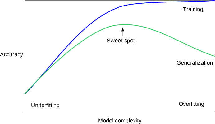
# ### 2.2 Generalization, Overfitting and Underfitting

# <img src="images/overfitting_underfitting_cartoon.png" alt="model_complexity" style="width: 50%;"/>

# #### 2.2.1 Relation of Model Complexity to Dataset Size

# ### 2.3 Supervised Machine Learning Algorithms
# #### 2.3.1 Some Sample Datasets

# - forge 데이터셋

# In[2]:


# generate dataset
X, y = mglearn.datasets.make_forge()
print("X.shape: {}".format(X.shape))
print("X:\n{}".format(X))
print("y.shape: {}".format(y.shape))
print("y:\n{}".format(y))

# plot dataset
plt.figure(figsize=(10, 5))
mglearn.discrete_scatter(X[:, 0], X[:, 1], y)
plt.legend(["Class 0", "Class 1"], loc=4)
plt.xlabel("First feature")
plt.ylabel("Second feature")
plt.show()


# - wave 데이터셋

# In[3]:


X, y = mglearn.datasets.make_wave(n_samples=40)
print("X.shape: {}".format(X.shape))
print("X:\n{}".format(X))
print("y.shape: {}".format(y.shape))
print("y:\n{}".format(y))

plt.figure(figsize=(10, 5))
plt.plot(X, y, 'o')
plt.ylim(-3, 3)
plt.xlabel("Feature")
plt.ylabel("Target")
plt.show()


# - Wisconsin Breast Cancer 데이터셋

# In[4]:


from sklearn.datasets import load_breast_cancer
cancer = load_breast_cancer()
print("cancer.keys(): {}".format(cancer.keys()))


# In[5]:


print("Shape of cancer data: {}".format(cancer.data.shape))


# In[6]:


print("Sample counts per class:\n{}".format(
      {n: v for n, v in zip(cancer.target_names, np.bincount(cancer.target))}
))


# In[7]:


print("Feature names:\n{}".format(cancer.feature_names))


# - Boston Housing 데이터셋

# In[8]:


from sklearn.datasets import load_boston
boston = load_boston()
print("boston.keys(): {}".format(boston.keys()))


# In[9]:


print("Feature Names: {}".format(boston.feature_names))
print("Feature Names: {}".format(boston.DESCR))


# In[10]:


print("Data shape: {}".format(boston.data.shape))
print("Target shape: {}".format(boston.target.shape))


# In[11]:


X, y = mglearn.datasets.load_extended_boston()
print("X.shape: {}".format(X.shape))


# ### 2.3.2 k-Nearest Neighbor
# #### k-Neighbors Classification

# In[12]:


plt.figure(figsize=(10, 5))
mglearn.plots.plot_knn_classification(n_neighbors=1)


# In[13]:


plt.figure(figsize=(10, 5))
mglearn.plots.plot_knn_classification(n_neighbors=3)


# In[14]:


from sklearn.model_selection import train_test_split
# X --> (26, 2)
# Y --> (26,)
X, y = mglearn.datasets.make_forge()

X_train, X_test, y_train, y_test = train_test_split(X, y, random_state=0)
print("X_train shape: {}".format(X_train.shape))
print("y_train shape: {}".format(y_train.shape))

print()

print("X_test shape: {}".format(X_test.shape))
print("y_test shape: {}".format(y_test.shape))


# In[15]:


from sklearn.neighbors import KNeighborsClassifier
clf = KNeighborsClassifier(n_neighbors=3)


# In[16]:


clf.fit(X_train, y_train)


# In[17]:


print("Test set predictions: {}".format(clf.predict(X_test)))


# In[18]:


print("Test set accuracy: {:.2f}".format(clf.score(X_test, y_test)))


# - clf.score() outputs 'R²' score
#   - 1.0 : Perfect Prediction
#   - 0.0 : Prediction to the mean of the given y values 
#   - $R^2 = 1 - {\frac{RSS}{TSS}}$
#     - RSS is the residual sum of squares $∑(y - f(x))²$
#     - TSS is the total sum of squares $∑(y - mean(y))²$.

# #### Analyzing KNeighborsClassifier

# In[19]:


fig, axes = plt.subplots(1, 3, figsize=(10, 3))

for n_neighbors, ax in zip([1, 3, 9], axes):
    # the fit method returns the object self, so we can instantiate
    # and fit in one line:
    clf = KNeighborsClassifier(n_neighbors=n_neighbors).fit(X, y)
    mglearn.plots.plot_2d_separator(clf, X, fill=True, eps=0.5, ax=ax, alpha=.4)
    mglearn.discrete_scatter(X[:, 0], X[:, 1], y, ax=ax)
    ax.set_title("{} neighbor(s)".format(n_neighbors))
    ax.set_xlabel("feature 0")
    ax.set_ylabel("feature 1")
axes[0].legend(loc=3)
plt.show()


# In[20]:


from sklearn.datasets import load_breast_cancer

cancer = load_breast_cancer()
X_train, X_test, y_train, y_test = train_test_split(
    cancer.data, 
    cancer.target, 
    stratify=cancer.target, 
    random_state=66
)

training_accuracy = []
test_accuracy = []
# try n_neighbors from 1 to 10
neighbors_settings = range(1, 11)

for n_neighbors in neighbors_settings:
    # build the model
    clf = KNeighborsClassifier(n_neighbors=n_neighbors)
    clf.fit(X_train, y_train)
    # record training set accuracy
    training_accuracy.append(clf.score(X_train, y_train))
    # record generalization accuracy
    test_accuracy.append(clf.score(X_test, y_test))

plt.figure(figsize=(8, 6), dpi=80, facecolor='w', edgecolor='k')
plt.plot(neighbors_settings, training_accuracy, label="training accuracy")
plt.plot(neighbors_settings, test_accuracy, label="test accuracy")
plt.ylabel("Accuracy")
plt.xlabel("n_neighbors")
plt.legend()
plt.show()


# #### k-Neighbors Regression

# In[21]:


mglearn.plots.plot_knn_regression(n_neighbors=1)


# In[22]:


mglearn.plots.plot_knn_regression(n_neighbors=3)


# In[23]:


from sklearn.neighbors import KNeighborsRegressor

X, y = mglearn.datasets.make_wave(n_samples=40)

# split the wave dataset into a training and a test set
X_train, X_test, y_train, y_test = train_test_split(X, y, random_state=0)

# instantiate the model and set the number of neighbors to consider to 3:
reg = KNeighborsRegressor(n_neighbors=3)
# fit the model using the training data and training targets:
reg.fit(X_train, y_train)


# In[24]:


print("Test set predictions:\n{}".format(reg.predict(X_test)))


# In[25]:


print("Test set R^2: {:.2f}".format(reg.score(X_test, y_test)))


# #### Analyzing KNeighborsRegressor

# In[26]:


fig, axes = plt.subplots(1, 3, figsize=(15, 4))
# create 1,000 data points, evenly spaced between -3 and 3
line = np.linspace(-3, 3, 1000).reshape(-1, 1)
for n_neighbors, ax in zip([1, 3, 9], axes):
    # make predictions using 1, 3, or 9 neighbors
    reg = KNeighborsRegressor(n_neighbors=n_neighbors)
    reg.fit(X_train, y_train)
    ax.plot(line, reg.predict(line))
    ax.plot(X_train, y_train, '^', c=mglearn.cm2(0), markersize=8)
    ax.plot(X_test, y_test, 'v', c=mglearn.cm2(1), markersize=8)

    ax.set_title(
        "{} neighbor(s)\n train score: {:.2f} test score: {:.2f}".format(
            n_neighbors, reg.score(X_train, y_train),
            reg.score(X_test, y_test)))
    ax.set_xlabel("Feature")
    ax.set_ylabel("Target")
axes[0].legend(["Model predictions", "Training data/target",
                "Test data/target"], loc="best")


# ##### Strengths, weaknesses, and parameters
# - Strengths
#   - 이해하기 쉽다.
#   - 많은 조정작업 없어도 좋은 성능을 보임.
#   - 더 복잡한 알고리즘을 적용해 보기 전에 시도해볼만한 알고리즘.
# 
# - Weaknesses
#   - 훈련데이터가 너무 많을 때 성능이 좋지 않음.
#   - 수백개 이상의 많은 특성을 지닌 데이터셋에 대해서는 성능이 좋지 않음.
#   - 희소 (특성값 대부분이 0) 데이터셋에 대해서도 성능이 좋지 않음.
#   - 데이터 전처리 작업이 중요 (3장 참고)

# ### 2.3.3 Linear Models
# #### Linear models for regression

# In[27]:


mglearn.plots.plot_linear_regression_wave()


# #### Linear Regression (a.k.a. Ordinary Least Squares)
# - with wave datasets

# In[28]:


from sklearn.linear_model import LinearRegression
X, y = mglearn.datasets.make_wave(n_samples=60)
X_train, X_test, y_train, y_test = train_test_split(X, y, random_state=42)

lr = LinearRegression().fit(X_train, y_train)


# In[29]:


print("lr.coef_: {}".format(lr.coef_))
print("lr.intercept_: {}".format(lr.intercept_))


# In[30]:


print("Training set score: {:.2f}".format(lr.score(X_train, y_train)))
print("Test set score: {:.2f}".format(lr.score(X_test, y_test)))


# - with boston datasets

# In[31]:


X, y = mglearn.datasets.load_extended_boston()
print("Data shape: {}".format(X.shape))
print("Target shape: {}".format(y.shape))


# In[32]:


X_train, X_test, y_train, y_test = train_test_split(X, y, random_state=0)
lr = LinearRegression().fit(X_train, y_train)


# In[33]:


print("Training set score: {:.2f}".format(lr.score(X_train, y_train)))
print("Test set score: {:.2f}".format(lr.score(X_test, y_test)))


# - 위와 같이 훈련데이터 셋에 대해서는 높은 정확도가 나오지만, 테스트데이터 셋에 대해서 낮은 정확도가 나오면 ---> Overfitting!!!
# - 단순 평균제곱오차 기반의 단순 선형 회귀 모델로는 이러한 Overfitting 문제를 해결하기 쉽지 않음

# ##### Ridge regression
# - 평균제곱오차 식에 $\alpha \sum_{j=1}^{m} w_{j}^{2}$항이 추가됨
#   - 위 항을 L2 Norm 이라고 함.
# - 가중치(w)에 대한 L2 규제 (L2 Regularization):
#   - 모든 가중치 값들을 가능한 0에 가깝게 되도록 조정 --> 기울기를 작게 만듦 --> 즉, 각각의 특성이 출력에 주는 영향을 최소한으로 만듦
#   - alpha: 규제의 강도 조정
#      - alpha 값이 커지면 규제가 강화됨
#      - alpha 값이 작으면 규제가 약화됨 (alpha = 0 --> 규제가 없음 --> 가중치 값의 자유도가 너무 높게됨 --> Overfitting 발생)

# In[34]:


from sklearn.linear_model import Ridge

ridge = Ridge().fit(X_train, y_train)
print("Training set score: {:.2f}".format(ridge.score(X_train, y_train)))
print("Test set score: {:.2f}".format(ridge.score(X_test, y_test)))


# In[35]:


ridge10 = Ridge(alpha=10).fit(X_train, y_train)
print("Training set score: {:.2f}".format(ridge10.score(X_train, y_train)))
print("Test set score: {:.2f}".format(ridge10.score(X_test, y_test)))


# In[36]:


ridge01 = Ridge(alpha=0.1).fit(X_train, y_train)
print("Training set score: {:.2f}".format(ridge01.score(X_train, y_train)))
print("Test set score: {:.2f}".format(ridge01.score(X_test, y_test)))


# In[37]:


plt.plot(ridge.coef_, 's', label="Ridge alpha=1")
plt.plot(ridge10.coef_, '^', label="Ridge alpha=10")
plt.plot(ridge01.coef_, 'v', label="Ridge alpha=0.1")

plt.plot(lr.coef_, 'o', label="LinearRegression")
plt.xlabel("Coefficient index")
plt.ylabel("Coefficient magnitude")
xlims = plt.xlim()
plt.hlines(0, xlims[0], xlims[1])
plt.xlim(xlims)
plt.ylim(-25, 25)
plt.legend()


# ##### Lasso
# - 평균제곱오차식에 $\alpha \sum_{j=1}^{m} |w_{j}|$ 항이 추가됨
#   - 위 항을 L1 노름이라고 함
# - 라쏘와 다른점
#   - 임의의 계수가 0이 되어 완전히 제거되는 특성이 생김
#   - 즉, 특성 선택(Feature Selection)이 자동으로 이루어짐 

# In[38]:


X, y = mglearn.datasets.make_wave(n_samples=60)
X_train, X_test, y_train, y_test = train_test_split(X, y, random_state=42)


# In[39]:


from sklearn.linear_model import Lasso

lasso = Lasso().fit(X_train, y_train)
print("Training set score: {:.2f}".format(lasso.score(X_train, y_train)))
print("Test set score: {:.2f}".format(lasso.score(X_test, y_test)))
print("Number of features used: {}".format(np.sum(lasso.coef_ != 0)))


# In[40]:


# we increase the default setting of "max_iter",
# otherwise the model would warn us that we should increase max_iter.
lasso001 = Lasso(alpha=0.01, max_iter=100000).fit(X_train, y_train)
print("Training set score: {:.2f}".format(lasso001.score(X_train, y_train)))
print("Test set score: {:.2f}".format(lasso001.score(X_test, y_test)))
print("Number of features used: {}".format(np.sum(lasso001.coef_ != 0)))


# In[41]:


lasso00001 = Lasso(alpha=0.0001, max_iter=100000).fit(X_train, y_train)
print("Training set score: {:.2f}".format(lasso00001.score(X_train, y_train)))
print("Test set score: {:.2f}".format(lasso00001.score(X_test, y_test)))
print("Number of features used: {}".format(np.sum(lasso00001.coef_ != 0)))


# In[42]:


plt.plot(lasso.coef_, 's', label="Lasso alpha=1")
plt.plot(lasso001.coef_, '^', label="Lasso alpha=0.01")
plt.plot(lasso00001.coef_, 'v', label="Lasso alpha=0.0001")

plt.plot(ridge01.coef_, 'o', label="Ridge alpha=0.1")

plt.legend(ncol=2, loc=(0, 1.05))
plt.ylim(-25, 25)
plt.xlabel("Coefficient index")
plt.ylabel("Coefficient magnitude")


# - Lasso 모델인 경우 많은 계수가 0이 되는 것을 알 수 있음
# - 반면, Ridge 모델인 경우 계수가 0이 되는 경우는 극히 드물다.

# #### Linear models for Classification (분류를 위한 선형 모델)

# - LogisticRegression & LinearSVC
#   - 기본적으로 L2 규제 사용
#   - 대표적인 선형 분류 모델
# - LinearSVC
#   - 서포트 벡터(Support Vector)
#     - 두 클래스 사이의 경계에 위치한 데이터 포인트
#     - 서포트 벡터 사이의 폭을 고려할 때 그러한 폭 중 가장 큰 폭을 가진 경계를 찾는 알고리즘
# ![](https://upload.wikimedia.org/wikipedia/commons/thumb/2/2a/Svm_max_sep_hyperplane_with_margin.png/330px-Svm_max_sep_hyperplane_with_margin.png)
# - with forge data

# In[43]:


from sklearn.linear_model import LogisticRegression
from sklearn.svm import LinearSVC

X, y = mglearn.datasets.make_forge()
print("Data shape: {}".format(X.shape))
print("Target shape: {}".format(y.shape))


# In[44]:


fig, axes = plt.subplots(1, 2, figsize=(10, 3))

for model, ax in zip([LinearSVC(), LogisticRegression()], axes):
    clf = model.fit(X, y)
    mglearn.plots.plot_2d_separator(clf, X, fill=False, eps=0.5, ax=ax, alpha=.7)
    mglearn.discrete_scatter(X[:, 0], X[:, 1], y, ax=ax)
    ax.set_title("{}".format(clf.__class__.__name__))
    ax.set_xlabel("Feature 0")
    ax.set_ylabel("Feature 1")
axes[0].legend()


# - LogisticRegression & LinearSVC
#   - C: 규제의 강도를 결정하는 매개변수
#     - default: 1.0
#     - Inverse of regularization strength; must be a positive float.
#     - 높은 C 값: 규제의 감소 --> 훈련 세트에 최대로 맞춤
#     - 낮은 C 값: 규제의 증대 --> 각각의 계수들을 최대로 0에 가깝게 만듦

# In[45]:


from sklearn.linear_model import LogisticRegression
from sklearn.svm import LinearSVC

X, y = mglearn.datasets.make_forge()

fig, axes = plt.subplots(1, 2, figsize=(10, 3))

for model, ax in zip([LinearSVC(C=0.01), LogisticRegression(C=0.01)], axes):
    clf = model.fit(X, y)
    mglearn.plots.plot_2d_separator(clf, X, fill=False, eps=0.5,
                                    ax=ax, alpha=.7)
    mglearn.discrete_scatter(X[:, 0], X[:, 1], y, ax=ax)
    ax.set_title("{}".format(clf.__class__.__name__))
    ax.set_xlabel("Feature 0")
    ax.set_ylabel("Feature 1")
axes[0].legend()


# In[46]:


mglearn.plots.plot_linear_svc_regularization()


# - with breast cancer data
#   - 차원이 높은 데이터에 대해서는 선형 모델을 사용할 때 Overfitting 주의

# In[47]:


from sklearn.datasets import load_breast_cancer
cancer = load_breast_cancer()
print("Shape of cancer data: {}".format(cancer.data.shape))

print()

X_train, X_test, y_train, y_test = train_test_split(cancer.data, cancer.target, stratify=cancer.target, random_state=42)
print("Shape of X_train: {}".format(X_train.shape))
print("Shape of X_test: {}".format(X_test.shape))

print()

logreg = LogisticRegression().fit(X_train, y_train)
print("Training set score: {:.3f}".format(logreg.score(X_train, y_train)))
print("Test set score: {:.3f}".format(logreg.score(X_test, y_test)))


# In[48]:


logreg100 = LogisticRegression(C=100).fit(X_train, y_train)
print("Training set score: {:.3f}".format(logreg100.score(X_train, y_train)))
print("Test set score: {:.3f}".format(logreg100.score(X_test, y_test)))


# In[49]:


logreg001 = LogisticRegression(C=0.01).fit(X_train, y_train)
print("Training set score: {:.3f}".format(logreg001.score(X_train, y_train)))
print("Test set score: {:.3f}".format(logreg001.score(X_test, y_test)))


# In[50]:


plt.plot(logreg.coef_.T, 'o', label="C=1")
plt.plot(logreg100.coef_.T, '^', label="C=100")
plt.plot(logreg001.coef_.T, 'v', label="C=0.001")
plt.xticks(range(cancer.data.shape[1]), cancer.feature_names, rotation=90)
xlims = plt.xlim()
plt.hlines(0, xlims[0], xlims[1])
plt.xlim(xlims)
plt.ylim(-5, 5)
plt.xlabel("Feature")
plt.ylabel("Coefficient magnitude")
plt.legend()


# - L1 규제 사용
#   - penalty = 'l1' 

# In[51]:


for C, marker in zip([0.001, 1, 100], ['o', '^', 'v']):
    lr_l1 = LogisticRegression(C=C, penalty="l1").fit(X_train, y_train)
    print("Training accuracy of L1 logreg with C={:.3f}: {:.2f}".format(C, lr_l1.score(X_train, y_train)))
    print("Test accuracy of l1 logreg with C={:.3f}: {:.2f}".format(C, lr_l1.score(X_test, y_test)))
    plt.plot(lr_l1.coef_.T, marker, label="C={:.3f}".format(C))
    print()

plt.xticks(range(cancer.data.shape[1]), cancer.feature_names, rotation=90)
xlims = plt.xlim()
plt.hlines(0, xlims[0], xlims[1])
plt.xlim(xlims)
plt.xlabel("Feature")
plt.ylabel("Coefficient magnitude")

plt.ylim(-5, 5)
plt.legend(loc=3)


# ##### Linear models for multiclass classification
# - 일대다 (one-vs.-rest) 방법
#   - 클래스의 개수 만큼 이진 분류기 생성
#   - 예측을 할 때에는 만들어진 모든 이진 분류기를 사용하여 가장 높은 점수를 내는 분류기의 클래스를 예측값으로 선택

# In[52]:


from sklearn.datasets import make_blobs

X, y = make_blobs(random_state=42)
print("Data shape: {}".format(X.shape))
print("Target shape: {}".format(y.shape))
print(y[0])
print(y[1])
print(y[2])

mglearn.discrete_scatter(X[:, 0], X[:, 1], y)
plt.xlabel("Feature 0")
plt.ylabel("Feature 1")
plt.legend(["Class 0", "Class 1", "Class 2"])


# In[53]:


linear_svm = LinearSVC().fit(X, y)
print("Coefficient shape: ", linear_svm.coef_.shape)
print("Intercept shape: ", linear_svm.intercept_.shape)


# - 각 세 개의 클래스 당 하나의 이진 분류기가 만들어짐
#   - (3, 2) 에서 각 행은 각 클래스에 대응하는 계수 백터
#   - (3,)은 각 클래스의 절편을 담은 1차원 벡터

# In[54]:


mglearn.discrete_scatter(X[:, 0], X[:, 1], y)
line = np.linspace(-15, 15)
for coef, intercept, color in zip(linear_svm.coef_, linear_svm.intercept_,
                                  mglearn.cm3.colors):
    plt.plot(line, -(line * coef[0] + intercept) / coef[1], c=color)
plt.ylim(-10, 15)
plt.xlim(-10, 8)
plt.xlabel("Feature 0")
plt.ylabel("Feature 1")
plt.legend(['Class 0', 'Class 1', 'Class 2', 'Line class 0', 'Line class 1', 'Line class 2'], loc=(1.01, 0.3))


# In[55]:


mglearn.plots.plot_2d_classification(linear_svm, X, fill=True, alpha=.7)
mglearn.discrete_scatter(X[:, 0], X[:, 1], y)
line = np.linspace(-15, 15)
for coef, intercept, color in zip(linear_svm.coef_, linear_svm.intercept_,
                                  mglearn.cm3.colors):
    plt.plot(line, -(line * coef[0] + intercept) / coef[1], c=color)
plt.legend(['Class 0', 'Class 1', 'Class 2', 'Line class 0', 'Line class 1',
            'Line class 2'], loc=(1.01, 0.3))
plt.xlabel("Feature 0")
plt.ylabel("Feature 1")


# #### Strengths, weaknesses and parameters
# - Linear Regression
#   - 특성 가중치 규제 강도 조정: alpha
#     - alpha가 높으면 규제를 강화함 --> 모델이 단순해짐
# - LinearSVC & LogisticRegression
#   - 특성 가중치 규제 강도 조정: C
#     - C가 낮으면 규제를 강화함 --> 모델이 단순해짐
# - 보통 alpha와 C는 로그스케일로 값을 정함
#   - 0.1, 1, 10 
# - L1 vs. L2
#   - 중요한 특성이 많지 않아서 몇몇 특성만 골라 활용하려고 하면 L1 규제 적당
#   - 모델의 해석이 중요할 때에도 L1 규제 사용
# - 대용량 데이터
#   - LogisticRegression 과 Ridge 에 solver='sag' 옵션 설정
#     - Stochastic Average Gradient Descent: 반복이 진행될 때 이전에 구한 모든 경사의 평균을 사용하여 계수를 갱신함
#   - SGDClassifier, SGDRegressor 사용

# ##### Method Chaining (메소드 연결)

# In[56]:


logreg = LogisticRegression()
logreg.fit(X_train, y_train)


# In[57]:


# instantiate model and fit it in one line
logreg = LogisticRegression().fit(X_train, y_train)


# In[58]:


logreg = LogisticRegression()
y_pred = logreg.fit(X_train, y_train).predict(X_test)


# In[59]:


y_pred = LogisticRegression().fit(X_train, y_train).predict(X_test)


# ### 2.3.4 Naive Bayes Classifiers
# - LogisticRegression 이나 LinearSVC보다 훈련 속도가 빠르지만 일반화 성능이 조금 떨어짐
# - scikit-learn 모델
#   - GaussianNB
#     - 연속 데이터에 적용
#   - BernoulliNB
#     - 이진 데이터에 적용
#   - MultinomialNB
#     - 카운트 데이터에 적용 
#     - 예를 들면, 문장에 나타난 단어의 횟수
# - 베이즈 정리
#   - $\displaystyle P(A∣B)= \frac{P(B∩A)}{P(B)}=\frac{P(A)P(B∣A)}{P(B)}$
#   ![!](https://upload.wikimedia.org/wikipedia/commons/thumb/1/18/Bayes%27_Theorem_MMB_01.jpg/440px-Bayes%27_Theorem_MMB_01.jpg)
#   - [Source: wikipedia]
#   <br/><br/>
# - 베이즈 분류
#   - 입력 데이터의 내용이 $X=(x_1, x_2, ..., x_p)$로 주어졌을 때 $Y=k$일 확률
#     - $\displaystyle P(Y = k ~|~ X_1 = x_1, X_2=x_2, ... , X_p = x_p)=P(Y = k) P(X_1 = x_1, X_2=x_2, ... , X_p = x_p~|~Y = k)$<br/><br/>
#   - 입력 데이터의 각 특성값의 조건부 분포가 서로 독립이라는 단순 베이즈 가정을 한다면
#     - $\displaystyle P(Y = k ~|~ X_1 = x_1, X_2=x_2, ... , X_p = x_p)=P(Y = k) \prod_{j=1}^{p}P(X_j = x_j~|~Y = k)$<br/><br/>
#   - 따라서, 입력 데이터의 내용이 $X=(x_1, x_2, ..., x_p)$로 주어졌을 때 $Y$ 예측 방법
#     - $\displaystyle argmax_{k\in Y} \big{(}P(Y = k) \prod_{j=1}^{p}P(X_j = x_j~|~Y = k)\big{)}$

# In[164]:


X = np.array([[0, 1, 0, 1],
              [1, 0, 1, 1],
              [0, 0, 0, 1],
              [1, 0, 1, 0]])
y = np.array([0, 1, 0, 1])


# In[165]:


counts = {}
for label in np.unique(y):
    # iterate over each class
    # count (sum) entries of 1 per feature
    counts[label] = X[y == label].sum(axis=0)
print("Feature counts:\n{}".format(counts))


# In[171]:


from sklearn.naive_bayes import BernoulliNB
clf = BernoulliNB()
clf.fit(X, y)
print("Prediction:", clf.predict([[0, 0, 0, 0]]))
print("Prediction:", clf.predict([[1, 1, 1, 1]])) 


# #### Strengths, weaknesses and parameters

# ### Decision trees

# In[62]:


mglearn.plots.plot_animal_tree()


# ##### Building decision trees

# In[63]:


mglearn.plots.plot_tree_progressive()


# ##### Controlling complexity of decision trees

# - Pre-pruning (사전 가지치기): 트리내 노드 생성을 사전에 중단
#   - scikit-learn 에서 지원하는 것
#   - 트리의 최대 깊이 제한
#   - 트리 내 리프 노드 개수 제한
#   - 분할 노드 개수 제한
# - Post-pruning (사후 가지치기) or Pruning: 트리의 노드를 만든 이후 데이터 포인트가 적은 노드를 삭제하거나 병합

# In[64]:


from sklearn.tree import DecisionTreeClassifier

cancer = load_breast_cancer()
print("Shape of cancer data: {}".format(cancer.data.shape))


# In[65]:


X_train, X_test, y_train, y_test = train_test_split(cancer.data, cancer.target, stratify=cancer.target, random_state=42)
print("Shape of X_train: {}".format(X_train.shape))
print("Shape of X_test: {}".format(X_test.shape))

print()

tree = DecisionTreeClassifier(random_state=0)
tree.fit(X_train, y_train)
print("Accuracy on training set: {:.3f}".format(tree.score(X_train, y_train)))
print("Accuracy on test set: {:.3f}".format(tree.score(X_test, y_test)))


# - 테스트 집합에 대한 0.937 정확도는 이전의 LogisticRegression의 테스트 집합 정확도보다 작음.

# - 트리의 깊이 제한
#   - max_depth=4

# In[66]:


tree = DecisionTreeClassifier(max_depth=4, random_state=0)
tree.fit(X_train, y_train)

print("Accuracy on training set: {:.3f}".format(tree.score(X_train, y_train)))
print("Accuracy on test set: {:.3f}".format(tree.score(X_test, y_test)))


# #### Analyzing Decision Trees

# In[67]:


from sklearn.tree import export_graphviz
export_graphviz(tree, 
                out_file="tree.dot", 
                class_names=["malignant", "benign"],
                feature_names=cancer.feature_names, 
                impurity=True, # When set to True, show the impurity (gini) at each node.
                filled=True # 노드의 분류 클래스가 구분되도록 색이 칠해짐
)


# In[68]:


import graphviz

with open("tree.dot") as f:
    dot_graph = f.read()
display(graphviz.Source(dot_graph))


# - 첫번째 루트 노드
#   - 악성 샘플: 159, 양성 샘플: 267
# - 루트 노드의 오른쪽 가지 노드
#   - 악성 샘플: 134, 양성 샘플: 8
# - 루트 노드의 왼쪽 가지 노드 
#   - 악성 샘플: 25, 양성 샘플: 259

# #### Feature Importance in trees
# - 특성 중요도 (Feature Impotance)
#   - 트리를 만드는 결정에 각 특성이 얼마나 중요한지를 평가
#     - 0: 해당 특성이 분류에 전혀 활용되지 않았음
#     - 1: 해당 특성이 분류를 하였고, 타깃 클래스를 정확하게 예측하였음을 나타냄

# In[69]:


print("Feature importances:\n{}".format(tree.feature_importances_))


# In[70]:


def plot_feature_importances_cancer(model):
    n_features = cancer.data.shape[1]
    plt.barh(range(n_features), model.feature_importances_, align='center')
    plt.yticks(np.arange(n_features), cancer.feature_names)
    plt.xlabel("Feature importance")
    plt.ylabel("Feature")
    plt.ylim(-1, n_features)
    plt.figure(figsize=(8, 6), dpi=80, facecolor='w', edgecolor='k')
    plt.show()

plot_feature_importances_cancer(tree)


# - 특성 중요도는 항상 양수이며, 어떤 클래스를 지지하는 지 알 수는 없다.
#   - 아래 예에서 X[1] 특성은 두 개 클래스를 동시에 지지함.

# In[71]:


tree = mglearn.plots.plot_tree_not_monotone()
display(tree)


# - Regression with DecisionTreeRegressor
# - plt.semilogy()
#   - Make a plot with log scaling on the `y` axis.

# In[72]:


import os

ram_prices = pd.read_csv(os.path.join(mglearn.datasets.DATA_PATH, "ram_price.csv"))
print(ram_prices.shape)
print(ram_prices.head(3))

plt.semilogy(ram_prices.date, ram_prices.price)
plt.xlabel("Year")
plt.ylabel("Price in $/Mbyte")


# In[73]:


from sklearn.tree import DecisionTreeRegressor
# use historical data to forecast prices after the year 2000
data_train = ram_prices[ram_prices.date < 2000]
data_test = ram_prices[ram_prices.date >= 2000]

print(data_train.shape)
print(data_train.head(3))

print()

print(data_test.shape)
print(data_test.head(3))


# In[74]:


# predict prices based on date
# np.newaxis 으로 새로운 demension 생성
temp_X_train = data_train.date
print(temp_X_train.shape)
print(temp_X_train[0])
print(temp_X_train[1])

print()

X_train = data_train.date[:, np.newaxis]
print(X_train.shape)
print(X_train[0])
print(X_train[1])

print()

# we use a log-transform to get a simpler relationship of data to target
y_train = np.log(data_train.price)
print(y_train.shape)
print(y_train[0])
print(y_train[1])


# - 날짜 대비 메모리 가격의 관계를 선형으로 변경하여 예측 성능을 높힘.

# In[75]:


X_test = data_test.date[:, np.newaxis]
y_test = np.log(data_test.price)


# In[76]:


tree = DecisionTreeRegressor().fit(X_train, y_train)
linear_reg = LinearRegression().fit(X_train, y_train)

# predict on all data (훈련 데이터와 테스트 데이터를 포함한 모든 데이터에 대하여 예측 수행)
X_all = ram_prices.date[:, np.newaxis]

pred_tree = tree.predict(X_all)
pred_lr = linear_reg.predict(X_all)

# undo log-transform
price_tree = np.exp(pred_tree)
price_lr = np.exp(pred_lr)


# In[77]:


plt.semilogy(data_train.date, data_train.price, label="Training data")
plt.semilogy(data_test.date, data_test.price, label="Test data")
plt.semilogy(ram_prices.date, price_tree, label="Tree prediction")
plt.semilogy(ram_prices.date, price_lr, label="Linear prediction")
plt.legend()


# - 위 트리 모델 훈련시에 모델 복잡도에 제한을 두지 않았음. 
#   - 훈련 데이터를 완벽하게 예측함 --> 과적합
# - 트리 모델을 사용한 테스트 시에 예측해야 할 값이 모델을 생성할 때 사용한 데이터 범위 밖에 존재할 때 트리는 적당하지 않음.

# #### Strengths, weaknesses and parameters

# - 트리 모델의 장점
#   - 만들어진 모델을 쉽게 시각화하고 이해할 수 있음.
#   - 각 특성은 개별적으로 다루어지기 때문에 특성의 정규화가 필요없음.
#     - 각 특성의 스케일이 서로 달라도 문제 없이 모델 학습이 이루어짐.<br/><br/>
# 
# - 트리 모델의 단점
#   - 사전 가지치기를 사용할 지라도 종종 과대적합되는 경향이 있음. --> 해결책: Ensemble

# ### 2.3.6 Ensembles of Decision Trees
# ##### Random forests
# ###### Building random forests
# ###### Analyzing random forests

# In[78]:


from sklearn.ensemble import RandomForestClassifier
from sklearn.datasets import make_moons

X, y = make_moons(n_samples=100, noise=0.25, random_state=3)

print("Data shape: {}".format(X.shape))
print("Target shape: {}".format(y.shape))

X_train, X_test, y_train, y_test = train_test_split(X, y, stratify=y, random_state=42)


# In[79]:


forest = RandomForestClassifier(n_estimators=5, random_state=2)
forest.fit(X_train, y_train)


# - RandomForestClassifier
#   - http://scikit-learn.org/stable/modules/generated/sklearn.ensemble.RandomForestClassifier.html
#   - 각 트리에 대해 독립적인 bootstrap sample 생성
#     - bootstrap samples
#       - n_samples 개의 데이터 포인트 중에서 무작위로 n_samples 개의 데이터를 추출 (하나의 샘플이 중복되어 추출 가능)
#   - n_estimators
#     - 생성할 트리의 개수    
#   - max_features
#     - 각 트리 노드에서 후보 특성을 무작위로 선정
#     - 그러한 선정 작업시에 몇 개의 특성까지 선정할지를 결정함
#     - 후보 특성을 선정하는 작업은 매 노드마다 반복 --> 각 노드는 서로 다른 후보 특성을 사용하게 됨
#     - max_features를 n_features로 설정하면 각 노드에서 모든 특성을 고려 --> 무작위성이 줄어들게 됨
#     - max_features를 1로 설정하면 각 노드에서 선택된 특성의 임계값만으로 분기 --> 트리의 깊이가 깊어짐
#     - 기본값: auto
#       - RandomForestClassifier: sqrt(n_features)
#       - RandomForestRegressor: n_features
#   - n_jobs
#     - 사용할 CPU 코어 수 지정
#     - n_jobs = -1 로 지정하면 컴퓨터의 모든 코어 사용
#   - random_state
#     - 서로 다른 random_state에 대해 전혀 다른 트리들이 생성
#   - max_depth
#     - 사전 가지치기 옵션
#   - min_samples_split: int, float, optional (default=2)
#     - The minimum number of samples required to split an internal node:
#     - If int, then consider min_samples_split as the minimum number.
#     - If float, then min_samples_split is a percentage and ceil(min_samples_split * n_samples) are the minimum number of samples for each split.

# In[80]:


mat = np.ones((2,3))
print(mat.shape)
print(mat)

print()

mat2 = mat.ravel()  # ravel: 얽힌 것을 풀다.
print(mat2.shape)
print(mat2)


# In[81]:


fig, axes = plt.subplots(2, 3, figsize=(20, 10))

for i, (ax, tree) in enumerate(zip(axes.ravel(), forest.estimators_)):
    ax.set_title("Tree {}".format(i))
    mglearn.plots.plot_tree_partition(X_train, y_train, tree, ax=ax)
    
mglearn.plots.plot_2d_separator(forest, X_train, fill=True, ax=axes[-1, -1], alpha=.4)
axes[-1, -1].set_title("Random Forest")
mglearn.discrete_scatter(X_train[:, 0], X_train[:, 1], y_train)


# In[82]:


X_train, X_test, y_train, y_test = train_test_split(cancer.data, cancer.target, random_state=0)

forest = RandomForestClassifier(n_estimators=100, random_state=0)
forest.fit(X_train, y_train)

print("Accuracy on training set: {:.3f}".format(forest.score(X_train, y_train)))
print("Accuracy on test set: {:.3f}".format(forest.score(X_test, y_test)))


# In[83]:


plot_feature_importances_cancer(forest)


# - 랜덤 포레스트를 만드는 무작위성
#   - 알고리즘이 가능성 있는 많은 경우를 고려할 수 있게 해줌
#   - 단일 트리 방식보다 더 넓은 시각으로 데이터를 바라볼 수 있게 해줌

# ###### Strengths, weaknesses, and parameters
# - 랜던 포레스트는 회귀와 분류에 있어서 가장 널리 사용되는 머신러닝 알고리즘
# - 대부분의 경우에 있어서 성능이 뛰어나고 매개변수 튜닝없이도 잘 작동
# - 데이터 feature개수가 많지만 (차원이 높고) 희소한 데이터에서는 성능이 낮음
# - 선형 모델보다 속도가 느리고 더 많은 메모리 사용
# - 가용한 시간과 메모리가 허용하는 한 n_estimators는 클수록 좋음 --> 더 많은 트리 사용

# #### Gradient Boosted Regression Trees (Gradient Boosting Machines)
# - 회귀와 분류 모두에 사용
#   - GradientBoostingClassifier
#   - GradientBoostingRegressor
# - 이전 트리의 예측과 타깃값 사이의 오차를 줄이는 방향으로 트리를 구성
#   - 경사 하강법을 사용하여 다음에 추가될 트리가 예측해야 할 값을 보정
# - 기본적으로 무작위성이 없으며, 강력한 사전 가지치기 사용
#   - 1~5 레벨 정도의 깊지 않은 트리 구성
#   - 메모리를 적게 사용하고 예측도 빠름
# - 많은 개수의 Weak Learner (얕은 트리의 간단한 모델)를 활용
# - 주요 파라미터: learning_rate, n_estimators
#   - learning_rate가 크면 이전 트리의 보정을 강하게 하기 때문에 더 복잡한 모델을 구성하게 됨.
#   - n_estimators 값을 키워서 앙상블 내에 트리의 개수를 증가시키는 것이 좋음.

# In[84]:


from sklearn.ensemble import GradientBoostingClassifier

X_train, X_test, y_train, y_test = train_test_split(cancer.data, cancer.target, random_state=0)

gbrt = GradientBoostingClassifier(random_state=0)
gbrt.fit(X_train, y_train)

print("Accuracy on training set: {:.3f}".format(gbrt.score(X_train, y_train)))
print("Accuracy on test set: {:.3f}".format(gbrt.score(X_test, y_test)))


# - GradientBoostingClassifier 파라미터 기본값
#   - max_depth=3 (트리 깊이 3)
#   - n_estimators = 100 (트리 100개)
#   - learning_rate = 0.1

# In[85]:


gbrt = GradientBoostingClassifier(random_state=0, max_depth=1)
gbrt.fit(X_train, y_train)

print("Accuracy on training set: {:.3f}".format(gbrt.score(X_train, y_train)))
print("Accuracy on test set: {:.3f}".format(gbrt.score(X_test, y_test)))


# In[86]:


gbrt = GradientBoostingClassifier(random_state=0, learning_rate=0.01)
gbrt.fit(X_train, y_train)

print("Accuracy on training set: {:.3f}".format(gbrt.score(X_train, y_train)))
print("Accuracy on test set: {:.3f}".format(gbrt.score(X_test, y_test)))


# In[87]:


gbrt = GradientBoostingClassifier(random_state=0, max_depth=1)
gbrt.fit(X_train, y_train)

plot_feature_importances_cancer(gbrt)


# - GradientBoostingClassifier에서는 일부 특성이 종종 완전히 무시됨

# ##### Strengths, weaknesses and parameters
# - GradientBoostingClassifier 방법
#   - 지도학습에서 가장 강력하고 널리 사용되는 모델 중 하나
#   - 단점
#     - 매개변수 조정 필요
#     - 훈련시간이 다소 길다.
#     - 특성들에 대해 희소한 고차원 데이터에서 잘 작동하지 않음
# <!-- more -->
# <br/><br/>
# - xgboost (https://xgboost.readthedocs.io) 사용 검토 필요
#   - 대용량 분산 처리 지원
#   - GPU 활용 플러그인 지원

# ### 2.3.7 Kernelized Support Vector Machines (커널 서포트 벡터 머신)
# - 입력 데이터로 부터 단순한 초평면(Hyperplane)으로 정의되지 않는 복잡한 모델을 구성할 수 있도록 확장된 모델
# #### Linear Models and Non-linear Features

# In[141]:


X, y = make_blobs(centers=4, random_state=8)
y = y % 2

mglearn.discrete_scatter(X[:, 0], X[:, 1], y)
plt.xlabel("Feature 0")
plt.ylabel("Feature 1")


# In[142]:


from sklearn.svm import LinearSVC
linear_svm = LinearSVC().fit(X, y)

mglearn.plots.plot_2d_separator(linear_svm, X)
mglearn.discrete_scatter(X[:, 0], X[:, 1], y)
plt.xlabel("Feature 0")
plt.ylabel("Feature 1")


# - 원본 데이터셋에 비선형 특성을 추가하여 선형모델(LinearSVC)을 그대로 사용하는 방법

# In[143]:


# add the squared first feature
# 모든 행(:)에 대해 1번째 열(1:)의 제곱 값을 덧붙임
X_new = np.hstack([X, X[:, 1:] ** 2])
print("X - Data shape: {}".format(X.shape))
print(X[0])
print(X[1])
print(X[2])
print()

print("X_new - Data shape: {}".format(X_new.shape))
print(X_new[0])
print(X_new[1])
print(X_new[2])


# In[144]:


from mpl_toolkits.mplot3d import Axes3D, axes3d
figure = plt.figure()
# visualize in 3D

ax = Axes3D(figure, elev=-152, azim=-26)

# plot first all the points with y==0, then all with y == 1
mask = y == 0
print(mask[0])
print(mask[1])
print(mask[2])

ax.scatter(X_new[mask, 0], X_new[mask, 1], X_new[mask, 2], c='b', cmap=mglearn.cm2, s=60, edgecolor='k')
ax.scatter(X_new[~mask, 0], X_new[~mask, 1], X_new[~mask, 2], c='r', marker='^', cmap=mglearn.cm2, s=60, edgecolor='k')
ax.set_xlabel("feature0")
ax.set_ylabel("feature1")
ax.set_zlabel("feature1 ** 2")


# In[145]:


linear_svm_3d = LinearSVC().fit(X_new, y)

coef, intercept = linear_svm_3d.coef_.ravel(), linear_svm_3d.intercept_

print("coef shape:", coef.shape)
print(coef)
print("intercept shape:", intercept.shape)
print(intercept)


# In[146]:


# show linear decision boundary
xx = np.linspace(X_new[:, 0].min() - 2, X_new[:, 0].max() + 2, 50)
yy = np.linspace(X_new[:, 1].min() - 2, X_new[:, 1].max() + 2, 50)
print("xx shape:", xx.shape)
print("yy shape:", xx.shape)
print(xx[0], xx[1], "...", xx[-1])
print(yy[0], yy[1], "...", yy[-1])

print()

XX, YY = np.meshgrid(xx, yy)
ZZ = (coef[0] * XX + coef[1] * YY + intercept) / -coef[2]
print("XX shape:", XX.shape)
print("YY shape:", YY.shape)
print("ZZ shape:", ZZ.shape)
print(XX[0])
print(XX[1])

print(YY[0])
print(YY[1])

print(ZZ[0])
print(ZZ[1])


# In[147]:


figure = plt.figure()
ax = Axes3D(figure, elev=-152, azim=-26)

ax.plot_surface(XX, YY, ZZ, rstride=8, cstride=8, alpha=0.3)
ax.scatter(X_new[mask, 0], X_new[mask, 1], X_new[mask, 2], c='b', cmap=mglearn.cm2, s=60, edgecolor='k')
ax.scatter(X_new[~mask, 0], X_new[~mask, 1], X_new[~mask, 2], c='r', marker='^', cmap=mglearn.cm2, s=60, edgecolor='k')

ax.set_xlabel("feature0")
ax.set_ylabel("feature1")
ax.set_zlabel("feature1 ** 2")


# In[95]:


# https://docs.scipy.org/doc/numpy-1.13.0/reference/generated/numpy.c_.html
type(np.c_)


# In[96]:


print(XX.ravel()[0], XX.ravel()[1], "...", XX.ravel()[-1])
print(YY.ravel()[0], YY.ravel()[1], "...", YY.ravel()[-1])
print(ZZ.ravel()[0], ZZ.ravel()[1], "...", ZZ.ravel()[-1])

print()

c = np.c_[XX.ravel(), YY.ravel(), ZZ.ravel()]
print(c.shape)
print(c[0])
print(c[1])
print(c[-1])


# - 특성 0과 특성 1에 투영한 결정 경계 (Decision Boundary) 도시화

# In[148]:


ZZ = YY ** 2
dec = linear_svm_3d.decision_function(np.c_[XX.ravel(), YY.ravel(), ZZ.ravel()])

plt.contourf(XX, YY, dec.reshape(XX.shape), levels=[dec.min(), 0, dec.max()], cmap=mglearn.cm2, alpha=0.5)
mglearn.discrete_scatter(X[:, 0], X[:, 1], y)
plt.xlabel("Feature 0")
plt.ylabel("Feature 1")


# #### The Kernel Trick
# - 원본 데이터 특성에 비선형 특성을 추가하여 선형모델을 강력하게 만드는 방법의 단점
#   - 어떤 특성을 선택하여 비선형 특성을 만들지 선택해야 하는 문제 발생
#   - 많은 비선형 특성 추가에 따른 연산 비용 증가
# - Kernel Trick (커널 기법)
#   - 실제로 데이터 특성을 확장하지 않고, 데이터 사이의 거리(폭)을 계산할 때 확장된 특성에 대한 데이터 포인트들의 거리를 계산
#   - 커널의 종류
#     - 다항식 커널
#       - 모든 원본 데이터 특성들에 대하여 가능한 조합을 지정된 차수까지 모두 계산
#         - 예: $특성1^2 \times 특성2^5$
#     - RBF (Radial Basis Function) or Gaussian (가우시안)
#       - 모든 원본 데이터 특성을 무한한 특성 공간에 매핑
#       - 즉, 모든 차수의 모든 다항식을 고려
#         - 일반적으로 고차항이 될 수록 특성의 중요도는 떨어지게됨
# <br/>
# <br/>
# 
# #### Understanding SVMs
# - Support Vectors
#   - 주어진 훈련 데이터들 중 두 클래스 사이의 경계에 위치한 데이터 포인트들 --> 결정 경계를 만드는데 영향을 주는 포인트들
#   - RBF 커널 (가우시안 커널) 에서의 데이터 포인트 $x_1$과 $x_2$ 사이 거리
#     - $k_{rbf}(x_1, x_2 )=exp(-\gamma||x_1 - x_2 ||^2 )$
#     - $\gamma$ : 가우시안 커널의 폭을 제어하는 매개변수

# In[149]:


from sklearn.svm import SVC

X, y = mglearn.tools.make_handcrafted_dataset()
print("X.shape:", X.shape)
print("y.shape:", y.shape)


# In[150]:


svm = SVC(kernel='rbf', C=10, gamma=0.1).fit(X, y)

mglearn.plots.plot_2d_separator(svm, X, eps=.5)
mglearn.discrete_scatter(X[:, 0], X[:, 1], y)

# plot support vectors
sv = svm.support_vectors_
dual_coef = svm.dual_coef_
print(sv)
print(dual_coef)

# class labels of support vectors are given by the sign of the dual coefficients
sv_labels = dual_coef.ravel() > 0
mglearn.discrete_scatter(sv[:, 0], sv[:, 1], sv_labels, s=15, markeredgewidth=3)
plt.xlabel("Feature 0")
plt.ylabel("Feature 1")


# #### Tuning SVM parameters (SVM 파라미터 튜닝)
# - SVC(kernel='rbf', C=10, gamma=0.1) 에서 각 매개변수 튜닝
#   - gamma
#     - 가우시안 커널 폭과 반비례
#     - 훈련 샘플 데이터가 미치는 영향의 범위 결정
#     - gamma값이 커짐 --> 가우시안 커널의 반경이 작아짐 --> 모델의 복잡도가 높아짐
#     - gamma값이 작아짐 --> 가우시안 커널의 반경이 커짐 --> 모델의 복잡도가 낮아짐
#   - C (Regulation, 규제 변수)
#     - C가 커짐 --> 모델 제약이 작아짐 --> 샘플 데이터가 모델에 많은 영향을 줌 --> 모델의 복잡도가 높아짐
#     - C가 작아짐 --> 모델 제약이 커짐 --> 샘플 데이터가 모델에 적은 영향을 줌 --> 모델의 복잡도가 낮아짐
#   - 즉...
#     - 모델 복잡도 증가 --> gamma값 증가 --> C값 증가
#     - 모델 복잡도 감소 --> gamma값 감소 --> C값 감소

# In[99]:


fig, axes = plt.subplots(3, 3, figsize=(15, 10))

for ax, C in zip(axes, [-1, 0, 3]):
    for a, gamma in zip(ax, range(-1, 2)):
        mglearn.plots.plot_svm(log_C=C, log_gamma=gamma, ax=a)
        
axes[0, 0].legend(["class 0", "class 1", "sv class 0", "sv class 1"],
                  ncol=4, loc=(.9, 1.2))


# - 유방암 데이터에 SVC 적용
#   - SVC의 매개변수 기본 값
#     - C=1.0
#     - gamma=1/n_features 

# In[152]:


X_train, X_test, y_train, y_test = train_test_split(cancer.data, cancer.target, random_state=0)

svc = SVC()
svc.fit(X_train, y_train)

print("Accuracy on training set: {:.2f}".format(svc.score(X_train, y_train)))
print("Accuracy on test set: {:.2f}".format(svc.score(X_test, y_test)))


# - 훈련 데이터에 대한 Scaling이 되어 있지 않음 --> 모델 성능 저하

# In[153]:


plt.boxplot(X_train, manage_xticks=False)
plt.yscale("symlog")
plt.xlabel("Feature index")
plt.ylabel("Feature magnitude")


# ##### Preprocessing data for SVMs

# - SVM에서는 특히 각 특성값의 범위가 비슷해지도록 정규화하는 것 매우 중요
# - 정규화 식
# $$\frac{X-min(X)}{max(X)-min(X)}$$

# In[155]:


print(X_train.shape)
# Compute the minimum value per feature on the training set
min_on_training = X_train.min(axis=0)
print(min_on_training.shape)

# Compute the range of each feature (max - min) on the training set
range_on_training = (X_train - min_on_training).max(axis=0)

# subtract the min, divide by range
# afterward, min=0 and max=1 for each feature
X_train_scaled = (X_train - min_on_training) / range_on_training
print("Minimum for each feature\n{}".format(X_train_scaled.min(axis=0)))
print("Maximum for each feature\n {}".format(X_train_scaled.max(axis=0)))


# - [NOTE] 테스트 데이터 세트에 대해서도 동일한 정규화를 하지만, 훈련 데이터 세트에서 계산된 최소값과 최대값과 해당 범위를 사용

# In[158]:


# use THE SAME transformation on the test set,
# using min and range of the training set. See Chapter 3 (unsupervised learning) for details.
X_test_scaled = (X_test - min_on_training) / range_on_training


# In[159]:


svc = SVC()
svc.fit(X_train_scaled, y_train)

print("Accuracy on training set: {:.3f}".format(svc.score(X_train_scaled, y_train)))
print("Accuracy on test set: {:.3f}".format(svc.score(X_test_scaled, y_test)))


# In[160]:


svc = SVC(C=1000)
svc.fit(X_train_scaled, y_train)

print("Accuracy on training set: {:.3f}".format(
    svc.score(X_train_scaled, y_train)))
print("Accuracy on test set: {:.3f}".format(svc.score(X_test_scaled, y_test)))


# #### Strengths, weaknesses and parameters
# - SVM 장점
#   - 다양한 데이터셋에 대해서도 잘 작동하는 강력한 모델
#   - 데이터의 특성이 몇 개 되지 않더라도 복잡한 결정 경계 생성 가능
# - SVM 단점
#   - 샘플 데이터 개수가 너무 많을 때 성능이 오히려 떨어질 수 있음
#   - 데이터 전처리와 매개변수 설정에 신경을 많이 써야 함

# ### 2.3.8 Neural Networks (Deep Learning)
# #### The Neural Network Model

# In[106]:


display(mglearn.plots.plot_logistic_regression_graph())


# In[107]:


display(mglearn.plots.plot_single_hidden_layer_graph())


# In[108]:


line = np.linspace(-3, 3, 100)
plt.plot(line, np.tanh(line), label="tanh")
plt.plot(line, np.maximum(line, 0), label="relu")
plt.legend(loc="best")
plt.xlabel("x")
plt.ylabel("relu(x), tanh(x)")


# In[109]:


mglearn.plots.plot_two_hidden_layer_graph()


# #### Tuning Neural Networks
# - MLPClassifier(solver='lbfgs', random_state=0, hidden_layer_sizes=(100, ), activation='tanh')
#   - hidden_layer_sizes 매개변수가 없을 때 기본적인 신경망 구조
#     - 기본: hidden layer 1개
#     - 기본: hidden unit 개수: 100개
#     - hidden_layer_sizes=(10, 10)
#       - hidden layer 2개
#       - hidden layer unit 수 - 각 층마다 10개씩
#   - activation
#     - 기본값: relu
#     - tanh
#   - solver (=optimizer)
#     - 기본값: adam
#       - 데이터의 스케일에 민감 --> 정규화 (평균 0, 분산 1) 중요
#     - lbfgs
#       - an optimizer in the family of quasi-Newton methods
#       - 대부분의 경우 안정적
#       - 대량의 데이터에 대한 많은 연산 필요
#     - sgd
#       - momentum 및 nesterov_momentum 매개변수 지정 필요
#       - momentum
#         - 새롭게 계산된 그레디언트에 대해 momentum 매개변수에 지정된 비율만큼만 반영 --> 관성 적용
#       - nesterov_momentum
#         - momentum 방식으로 구한 그레디언트를 이전 그레디언트로 가정
#         - 한번 더 momentum 방식을 적용하여 새로운 그레디언트 계산
#   - batch_size : int, optional, default ‘auto’
#     - Size of minibatches for stochastic optimizers. 
#     - If the solver is ‘lbfgs’, the classifier will not use minibatch. 
#     - When set to “auto”, batch_size=min(200, n_samples)

# In[110]:


from sklearn.neural_network import MLPClassifier
from sklearn.datasets import make_moons

X, y = make_moons(n_samples=100, noise=0.25, random_state=3)

X_train, X_test, y_train, y_test = train_test_split(X, y, stratify=y, random_state=42)

mlp = MLPClassifier(solver='lbfgs', random_state=0).fit(X_train, y_train)
mglearn.plots.plot_2d_separator(mlp, X_train, fill=True, alpha=.3)
mglearn.discrete_scatter(X_train[:, 0], X_train[:, 1], y_train)
plt.xlabel("Feature 0")
plt.ylabel("Feature 1")


# In[111]:


mlp = MLPClassifier(solver='lbfgs', random_state=0, hidden_layer_sizes=[10])
mlp.fit(X_train, y_train)
mglearn.plots.plot_2d_separator(mlp, X_train, fill=True, alpha=.3)
mglearn.discrete_scatter(X_train[:, 0], X_train[:, 1], y_train)
plt.xlabel("Feature 0")
plt.ylabel("Feature 1")


# In[112]:


# using two hidden layers, with 10 units each
mlp = MLPClassifier(solver='lbfgs', random_state=0, hidden_layer_sizes=[10, 10])
mlp.fit(X_train, y_train)
mglearn.plots.plot_2d_separator(mlp, X_train, fill=True, alpha=.3)
mglearn.discrete_scatter(X_train[:, 0], X_train[:, 1], y_train)
plt.xlabel("Feature 0")
plt.ylabel("Feature 1")


# In[113]:


# using two hidden layers, with 10 units each, now with tanh nonlinearity.
mlp = MLPClassifier(solver='lbfgs', activation='tanh', random_state=0, hidden_layer_sizes=[10, 10])
mlp.fit(X_train, y_train)
mglearn.plots.plot_2d_separator(mlp, X_train, fill=True, alpha=.3)
mglearn.discrete_scatter(X_train[:, 0], X_train[:, 1], y_train)
plt.xlabel("Feature 0")
plt.ylabel("Feature 1")


# - L2 규제 사용
#   - alpha 매개변수 사용
#     - 기본값: 0.00001

# In[114]:


fig, axes = plt.subplots(2, 4, figsize=(20, 8))
for axx, n_hidden_nodes in zip(axes, [10, 100]):
    for ax, alpha in zip(axx, [0.0001, 0.01, 0.1, 1]):
        mlp = MLPClassifier(solver='lbfgs', random_state=0, hidden_layer_sizes=[n_hidden_nodes, n_hidden_nodes],
                            alpha=alpha)
        mlp.fit(X_train, y_train)
        mglearn.plots.plot_2d_separator(mlp, X_train, fill=True, alpha=.3, ax=ax)
        mglearn.discrete_scatter(X_train[:, 0], X_train[:, 1], y_train, ax=ax)
        ax.set_title("n_hidden=[{}, {}]\nalpha={:.4f}".format(n_hidden_nodes, n_hidden_nodes, alpha))


# In[115]:


fig, axes = plt.subplots(2, 4, figsize=(20, 8))
for i, ax in enumerate(axes.ravel()):
    mlp = MLPClassifier(solver='lbfgs', random_state=i, hidden_layer_sizes=[100, 100])
    mlp.fit(X_train, y_train)
    mglearn.plots.plot_2d_separator(mlp, X_train, fill=True, alpha=.3, ax=ax)
    mglearn.discrete_scatter(X_train[:, 0], X_train[:, 1], y_train, ax=ax)
    ax.set_title("random_state={}".format(i))


# In[116]:


print("Cancer data per-feature maxima:\n{}".format(cancer.data.max(axis=0)))


# In[117]:


X_train, X_test, y_train, y_test = train_test_split(cancer.data, cancer.target, random_state=0)

mlp = MLPClassifier(random_state=42)
mlp.fit(X_train, y_train)

print("Accuracy on training set: {:.2f}".format(mlp.score(X_train, y_train)))
print("Accuracy on test set: {:.2f}".format(mlp.score(X_test, y_test)))


# - 유방암 데이터에 대한 정규화

# In[118]:


# compute the mean value per feature on the training set
mean_on_train = X_train.mean(axis=0)
# compute the standard deviation of each feature on the training set
std_on_train = X_train.std(axis=0)

# subtract the mean, and scale by inverse standard deviation
# afterward, mean=0 and std=1
X_train_scaled = (X_train - mean_on_train) / std_on_train
# use THE SAME transformation (using training mean and std) on the test set
X_test_scaled = (X_test - mean_on_train) / std_on_train

mlp = MLPClassifier(random_state=0)
mlp.fit(X_train_scaled, y_train)

print("Accuracy on training set: {:.3f}".format(mlp.score(X_train_scaled, y_train)))
print("Accuracy on test set: {:.3f}".format(mlp.score(X_test_scaled, y_test)))


# - adam optimizer에서 200번 정도의 iteration으로는 converge 시키기 부족함 --> max_iter 값 증가 필요

# In[119]:


mlp = MLPClassifier(max_iter=1000, random_state=0)
mlp.fit(X_train_scaled, y_train)

print("Accuracy on training set: {:.3f}".format(mlp.score(X_train_scaled, y_train)))
print("Accuracy on test set: {:.3f}".format(mlp.score(X_test_scaled, y_test)))


# - L2 규제 (일반화 성능 증대)
#   - alpha = 1.0

# In[120]:


mlp = MLPClassifier(max_iter=1000, alpha=1.0, random_state=0)
mlp.fit(X_train_scaled, y_train)

print("Accuracy on training set: {:.3f}".format(mlp.score(X_train_scaled, y_train)))
print("Accuracy on test set: {:.3f}".format(mlp.score(X_test_scaled, y_test)))


# - 입력과 첫번째 hidden layer 사이의 학습된 가중치 값 시각화
#   - 작은 가중치를 지닌 특성이 덜 중요하다고 해석 가능

# In[121]:


plt.figure(figsize=(20, 5))
plt.imshow(mlp.coefs_[0], interpolation='none', cmap='viridis')
plt.yticks(range(30), cancer.feature_names)
plt.xlabel("Columns in weight matrix")
plt.ylabel("Input feature")
plt.colorbar()


# #### Strengths, weaknesses and parameters
# - MLPClassifier의 한계
#   - CNN, RNN 등의 복잡한 딥러닝 신경망 구성할 수 없음
#     - scikit-learn 에서는 아직 CNN과 RNN을 지원하지 않음 
#   - 이러한 복잡한 딥러닝 신경망 구성은 keras 또는 tensorflow 활용 필요함
# - 신경망의 장점
#   - 많은 응용에서 최고의 모델로 평가받고 있음
#   - 대량의 데이터에 내재된 정보를 잡아내면서 복잡한 모델 구성 가능
#   - 충분한 연산 시간과 데이터를 주고 매개변수를 세심하게 조정하면 최고의 성능 발휘 가능
# - 신견망의 단점
#   - 학습 시간이 오래 걸림
#   - 데이터 전처리 중요
#     - 모든 특성이 동일한 범위를 지닌 데이터에 잘 작동

# #### Estimating complexity in neural networks
# - 일반적인 학습 모델 구성 방법
#   - 처음에는 한 개 또는 두 개의 은닉층으로 시작하면서 은닉층의 수를 늘려나감
#   - 각 은닉층의 유닛의 개수는 보통 입력 틍성의 수와 비슷하게 설정
#   - 일단 충분히 과대적합이 될 정도로 큰 신경망 모델을 구성
#   - 이후 alpha 값을 증가시키며 규제(Regularization)의 강도를 높힘
# <br/>  
# - 모델 구성 요성
#   - 층의 개수
#   - 층당 유닛 개수
#   - 가중치 초기값
#   - 규제의 강도
#   - 비활성화 함수 (relu, tanh, ...)
#   - 학습 알고리즘 (즉, solver)
#     - adam, sgd, lbfgs

# ### 2.4 Uncertainty estimates from classifiers
# - 불확실성 추정
#   - 분류모델이 예측한 분류 클래스가 얼마나 정확한 지 판단 필요
#   - 예를 들어, 암진단 응용에서 거짓 양성(False Positive) 분류는 환자에게 추가 진료를 요구하겠지만, 거짓 음성(False Negative) 분류는 심각한 질병을 치료하지 못하게 할 수 있음.
# <br/>
# - scikit-learn에서 제공하는 불확실성 추정 함수
#   - decision_function
#   - predict_prob

# In[143]:


from sklearn.ensemble import GradientBoostingClassifier
from sklearn.datasets import make_circles

X, y = make_circles(noise=0.25, factor=0.5, random_state=1)

print("Data shape: {}".format(X.shape))
print("Target shape: {}".format(y.shape))

print()

# we rename the classes "blue" and "red" for illustration bpurposes:
y_named = np.array(["blue", "red"])[y]
print("Named Target shape: {}".format(y_named.shape))
print(y[0], y_named[0])
print(y[1], y_named[1])
print(y[2], y_named[2])


# In[144]:


# we can call train_test_split with arbitrarily many arrays;
# all will be split in a consistent manner
X_train, X_test, y_train_named, y_test_named, y_train, y_test = train_test_split(X, y_named, y, random_state=0)

# build the gradient boosting model
gbrt = GradientBoostingClassifier(random_state=0)
gbrt.fit(X_train, y_train_named)


# #### 2.4.1 The Decision Function
# - decision_function 반환값
#   - 주어진 데이터 포인트 샘플당 하나의 실수값 반환
#   - 주어진 데이터 포인트가 양성 클래스인 1에 속한다고 믿는 정도
#   - 반환값의 부호
#     - 양수: 양성 클래스 (1)
#     - 음수: 음성 클래스 (0)

# In[145]:


print("X_test.shape: {}".format(X_test.shape))

print()

print("Decision function shape: {}".format(gbrt.decision_function(X_test).shape))

print()

print("Decision function:\n{}".format(gbrt.decision_function(X_test)))


# In[146]:


print("Thresholded decision function:\n{}".format(gbrt.decision_function(X_test) > 0))
print("Predictions:\n{}".format(gbrt.predict(X_test)))


# In[150]:


# make the boolean True/False into 0 and 1
greater_zero = (gbrt.decision_function(X_test) > 0).astype(int)
print(greater_zero)
print()

# use 0 and 1 as indices into classes_
print(gbrt.classes_)
pred = gbrt.classes_[greater_zero]

print(pred)

print()

# pred is the same as the output of gbrt.predict
print("pred is equal to predictions: {}".format(np.all(pred == gbrt.predict(X_test))))


# In[151]:


decision_function = gbrt.decision_function(X_test)
print("Decision function minimum: {:.2f} maximum: {:.2f}".format(np.min(decision_function), np.max(decision_function)))


# In[152]:


fig, axes = plt.subplots(1, 2, figsize=(13, 5))
mglearn.tools.plot_2d_separator(gbrt, X, ax=axes[0], alpha=.4, fill=True, cm=mglearn.cm2)
scores_image = mglearn.tools.plot_2d_scores(gbrt, X, ax=axes[1], alpha=.4, cm=mglearn.ReBl)

for ax in axes:
    # plot training and test points
    mglearn.discrete_scatter(X_test[:, 0], X_test[:, 1], y_test, markers='^', ax=ax)
    mglearn.discrete_scatter(X_train[:, 0], X_train[:, 1], y_train, markers='o', ax=ax)
    ax.set_xlabel("Feature 0")
    ax.set_ylabel("Feature 1")
cbar = plt.colorbar(scores_image, ax=axes.tolist())
cbar.set_alpha(1)
cbar.draw_all()
axes[0].legend(["Test class 0", "Test class 1", "Train class 0", "Train class 1"], ncol=4, loc=(.1, 1.1))


# - 왼쪽 그래프: 결정 경계
# - 오른쪽 그래프: decision_function의 값을 색으로 표현

# #### 2.4.2 Predicting Probabilities
# - predict_proba
#   - 각 분류 클래스에 대한 확률값 반환
#   - 반환값의 shape는 항상 (n_samples, 2)
#     - 각 샘플당 첫번째 원소는 첫번째 클래스의 예측 확률, 두번째 원소는 두번째 클래스의 예측 확률
#     - 두 원소 값의 합은 항상 1.0
#   - overfitting 된 복잡도가 높은 모델에서는 각 클래스에 대한 예측 확실성이 높음 (즉, 예측 확신이 강함)
#   - 일반적으로 복잡도가 낮은 모델은 예측에 대한 불확실성이 높음 (즉, 예측 확신이 약함)
# - 불확실의 정도와 모델의 정확도가 동일 --> 보정(Calibration)이 잘 되었다고 판단
#   - 보정이 잘 된 모델에서 70% 확신을 지닌 예측은 70%의 정확도를 냄

# In[153]:


print("Shape of probabilities: {}".format(gbrt.predict_proba(X_test).shape))

print()

# show the first few entries of predict_proba
print("Predicted probabilities:\n{}".format(gbrt.predict_proba(X_test)))


# In[132]:


fig, axes = plt.subplots(1, 2, figsize=(13, 5))
    
mglearn.tools.plot_2d_separator(gbrt, X, ax=axes[0], alpha=.4, fill=True, cm=mglearn.cm2)
scores_image = mglearn.tools.plot_2d_scores(gbrt, X, ax=axes[1], alpha=.5, cm=mglearn.ReBl, function='predict_proba')

for ax in axes:
    # plot training and test points
    mglearn.discrete_scatter(X_test[:, 0], X_test[:, 1], y_test, markers='^', ax=ax)
    mglearn.discrete_scatter(X_train[:, 0], X_train[:, 1], y_train, markers='o', ax=ax)
    ax.set_xlabel("Feature 0")
    ax.set_ylabel("Feature 1")
# don't want a transparent colorbar
cbar = plt.colorbar(scores_image, ax=axes.tolist())
cbar.set_alpha(1)
cbar.draw_all()
axes[0].legend(["Test class 0", "Test class 1", "Train class 0", "Train class 1"], ncol=4, loc=(.1, 1.1))


# - 많은 모델에 대한 불확실성 추정 도표
#   - http://bit.ly/2cqCYx6

# ![classifier_comparison](images/classifier_comparison.png)

# #### 2.4.3 Uncertainty in multi-class classification

# In[156]:


from sklearn.datasets import load_iris

iris = load_iris()
X_train, X_test, y_train, y_test = train_test_split(iris.data, iris.target, random_state=42)

gbrt = GradientBoostingClassifier(learning_rate=0.01, random_state=0)
gbrt.fit(X_train, y_train)


# In[157]:


print("Decision function shape: {}".format(gbrt.decision_function(X_test).shape))
# plot the first few entries of the decision function
print("Decision function:\n{}".format(gbrt.decision_function(X_test)[:6, :]))


# In[158]:


print("Argmax of decision function:\n{}".format(np.argmax(gbrt.decision_function(X_test), axis=1)))
print("Predictions:\n{}".format(gbrt.predict(X_test)))


# In[159]:


# show the first few entries of predict_proba
print("Predicted probabilities:\n{}".format(gbrt.predict_proba(X_test)[:6]))
# show that sums across rows are one
print("Sums: {}".format(gbrt.predict_proba(X_test)[:6].sum(axis=1)))


# In[160]:


print("Argmax of predicted probabilities:\n{}".format(np.argmax(gbrt.predict_proba(X_test), axis=1)))
print("Predictions:\n{}".format(gbrt.predict(X_test)))


# In[163]:


logreg = LogisticRegression()

# represent each target by its class name in the iris dataset
named_target = iris.target_names[y_train]
logreg.fit(X_train, named_target)
print("unique classes in training data: {}".format(logreg.classes_))

print()

print("predictions: {}".format(logreg.predict(X_test)[:10]))

print()

argmax_dec_func = np.argmax(logreg.decision_function(X_test), axis=1)
print("argmax of decision function: {}".format(argmax_dec_func[:10]))

print()

print("argmax combined with classes_: {}".format(logreg.classes_[argmax_dec_func][:10]))


# ### 2.5 Summary and Outlook
# - 최근접 이웃
# - 선형 모델
# - 나이브 베이즈
# - 결정 트리
# - 랜덤 포레스트
# - 그레디언트 부스팅 결정 트리
# - 서포트 벡터 머신
# - 신경망