![]() # # Isothermal Flash and the Rachford-Rice Equation
# ## Summary
#
# This [Jupyter notebook](http://jupyter.org/notebook.html) illustrates the use of the Rachford-Rice equation solve the material balances for an isothermal flash of an ideal mixture. The video is used with permission from [learnCheme.com](http://learncheme.ning.com/), a project at the University of Colorado funded by the National Science Foundation and the Shell Corporation.
# ## Derivation of the Rachford-Rice Equation
#
# The derivation of the Rachford-Rice equation is a relatively straightford application of component material balances and Raoult's law for an ideal solution.
# In[1]:
from IPython.display import YouTubeVideo
YouTubeVideo("ACxOiXWq1SQ",560,315,rel=0)
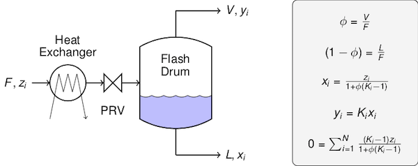
# The quantities, definitions, and equations are summarized in the following figure.
#
# 
#
# To sketch the derivation, we begin with the overall constraint on the liquid
# phase and vapor phase mole fractions $x_1 + x_2 + \cdots + x_N = 1$ and $y_1 + y_2 + \cdots + y_N = 1$. Subtracting the first from the second we find
#
# $$\sum_{n=1}^N (y_n - x_n) = 0$$
#
# This doesn't look like much, but it turns out to be the essential trick in the development.
#
# Next we need expressions for $y_n$ and $x_n$ to substitute into terms in the sum. We get these by solving the component material balance and equilibrium equations for $y_n$ and $x_n$. For each species we write a material balance
#
# $$L x_n + V y_n = F z_n$$
#
# Dividing through by the feedrate we get a parameter $\phi = \frac{V}{L}$ denoting the fraction of the feedstream that leaves the flash unit in the vapor stream, the remaining fraction $1-\phi$ leaving in the liquid stream. With this notation the material balance becomes
#
# $$(1-\phi)x_n + \phi y_n = z_n$$
#
# for each species.
#
# The second equation is
#
# $$y_n = K_n x_n$$
#
# where the 'K-factor' for an ideal solution is given by Raoult's law
#
# $$K_n = \frac{P_n^{sat}(T)}{P}$$
#
# The K-factor depends on the operating pressure and temperature of the flash unit. Solving the material balance and equilibrium equations gives
#
# $$x_n = \frac{z_n}{1 + \phi(K_n - 1)}$$
#
# $$y_n = \frac{K_n z_n}{1 + \phi(K_n - 1)}$$
#
# so that the difference $y_n - x_n$ is given by
#
# $$y_n - x_n = \frac{(K_n - 1)z_n}{1 + \phi(K_n - 1)}$$
#
# Substitution leads to the Rachford-Rice equation
#
# $$\sum_{n=1}^{N} \frac{(K_n - 1)z_n}{1 + \phi(K_n - 1)} = 0 $$
#
# This equation can be used to solve a variety of vapor-liquid equilibrium problems as outline in the following table.
# ## Problem Classification
#
# | Problem Type | zi's | T | P | φ | Action |
# | -----------: | :-----: | :-----: | :-----: | :-----: | :----: |
# | Bubble Point | ✓ | unknown | ✓ | 0 | Set xi = zi. Solve for T and yi's |
# | Bubble Point | ✓ | ✓ | unknown | 0 | Set xi = zi. Solve for P and yi's |
# | Dew Point | ✓ | unknown | ✓ | 1 | Set yi = zi. Solve for T and xi's |
# | Dew Point | ✓ | ✓ | unknown | 1 | Set yi = zi. Solve for P and xi's |
# | Isothermal Flash | ✓ | ✓ | ✓ | unknown | Solve for φ, xi's, and yi's |
#
# ## Isothermal Flash of a Binary Mixture
#
# Problem specifications
# In[1]:
import numpy as np
import matplotlib.pyplot as plt
get_ipython().run_line_magic('matplotlib', 'inline')
# In[2]:
A = 'acetone'
B = 'ethanol'
P = 760
T = 65
z = dict()
z[A] = 0.6
z[B] = 1 - z[A]
# Compute the K-factors for the given operating conditions
# In[3]:
# Antoine's equations. T [deg C], P [mmHg]
Psat = dict()
Psat[A] = lambda T: 10**(7.02447 - 1161.0/(224 + T))
Psat[B] = lambda T: 10**(8.04494 - 1554.3/(222.65 + T))
# Compute K-factors
K = dict()
K[A] = Psat[A](T)/P
K[B] = Psat[B](T)/P
print("Pressure {:6.2f} [mmHg]".format(P))
print("Temperature {:6.2f} [deg C]".format(T))
print("K-factors:")
for n in Psat:
print(" {:s} {:7.3f}".format(n,K[n]))
# Rachford-Rice equation
# In[4]:
def RR(phi):
return (K[A]-1)*z[A]/(1 + phi*(K[A]-1)) + (K[B]-1)*z[B]/(1 + phi*(K[B]-1))
phi = np.linspace(0,1)
plt.plot(phi,[RR(phi) for phi in phi])
plt.xlabel('Vapor Fraction phi')
plt.title('Rachford-Rice Equation')
plt.grid();
# Finding roots of the Rachford-Rice equation
# In[5]:
from scipy.optimize import brentq
phi = brentq(RR,0,1)
print("Vapor Fraction {:6.4f}".format(phi))
print("Liquid Fraction {:6.4f}".format(1-phi))
# Compositions
# In[6]:
x = dict()
y = dict()
print("Component z[n] x[n] y[n]")
for n in [A,B]:
x[n] = z[n]/(1 + phi*(K[n]-1))
y[n] = K[n]*x[n]
print("{:10s} {:6.4n} {:6.4f} {:6.4f}".format(n,z[n],x[n],y[n]))
# ## Multicomponent Mixtures
# In[7]:
P = 760
T = 65
z = dict()
z['acetone'] = 0.6
z['benzene'] = 0.01
z['toluene'] = 0.01
z['ethanol'] = 1 - sum(z.values())
# In[8]:
Psat = dict()
Psat['acetone'] = lambda T: 10**(7.02447 - 1161.0/(224 + T))
Psat['benzene'] = lambda T: 10**(6.89272 - 1203.531/(219.888 + T))
Psat['ethanol'] = lambda T: 10**(8.04494 - 1554.3/(222.65 + T))
Psat['toluene'] = lambda T: 10**(6.95805 - 1346.773/(219.693 + T))
K = {n : lambda P,T,n=n: Psat[n](T)/P for n in Psat}
print("Pressure {:6.2f} [mmHg]".format(P))
print("Temperature {:6.2f} [deg C]".format(T))
print("K-factors:")
for n in K:
print(" {:s} {:7.3f}".format(n,K[n](P,T)))
# In[9]:
def RR(phi):
return sum([(K[n](P,T)-1)*z[n]/(1 + phi*(K[n](P,T)-1)) for n in K.keys()])
phi = np.linspace(0,1)
plt.plot(phi,[RR(phi) for phi in phi])
plt.xlabel('Vapor Fraction phi')
plt.title('Rachford-Rice Equation')
plt.grid();
# In[10]:
from scipy.optimize import brentq
phi = brentq(RR,0,1)
print("Vapor Fraction {:6.4f}".format(phi))
print("Liquid Fraction {:6.4f}".format(1-phi))
# In[11]:
x = {n: z[n]/(1 + phi*(K[n](P,T)-1)) for n in z}
y = {n: K[n](P,T)*z[n]/(1 + phi*(K[n](P,T)-1)) for n in z}
print("Component z[n] x[n] y[n]")
for n in z.keys():
print("{:10s} {:6.4f} {:6.4f} {:6.4f}".format(n,z[n],x[n],y[n]))
# [Experiments](http://en.wikipedia.org/wiki/MythBusters_%282005_season%29#Bottle_Rocket_Blast-Off) suggest the bursting pressure of a 2 liter soda bottle is 150 psig.
# ## Exercises
# ### Design of a Carbonated Beverage
#
# The purpose of carbonating beverages is to provide a positive pressure inside the package to keep out oxygen and other potential contaminants. The burst pressure of 2 liter soda bottles [has been measured to be 150 psig](http://en.wikipedia.org/wiki/MythBusters_%282005_season%29#Bottle_Rocket_Blast-Off) (approx. 10 atm). For safety, suppose you want the bottle pressure to be no more than 6 atm gauge on a hot summer day in Arizona (say 50 °C, ) and yet have at least 0.5 atm of positive gauge pressure at 0 °C. Assuming your beverage is a mixture of CO2 and water, is it possible to meet this specification? What concentration (measured in g of CO2 per g of water) would you recommend?
# In[ ]:
#
# < [Bubble and Dew Points for Multicomponent Mixtures](http://nbviewer.jupyter.org/github/jckantor/CBE20255/blob/master/notebooks/07.08-Bubble-and-Dew-Points-for-Multicomponent-Mixtures.ipynb) | [Contents](toc.ipynb) | [Binary Distillation with McCabe-Thiele](http://nbviewer.jupyter.org/github/jckantor/CBE20255/blob/master/notebooks/07.10-Binary-Distillation-with-McCabe-Thiele.ipynb) >
# # Isothermal Flash and the Rachford-Rice Equation
# ## Summary
#
# This [Jupyter notebook](http://jupyter.org/notebook.html) illustrates the use of the Rachford-Rice equation solve the material balances for an isothermal flash of an ideal mixture. The video is used with permission from [learnCheme.com](http://learncheme.ning.com/), a project at the University of Colorado funded by the National Science Foundation and the Shell Corporation.
# ## Derivation of the Rachford-Rice Equation
#
# The derivation of the Rachford-Rice equation is a relatively straightford application of component material balances and Raoult's law for an ideal solution.
# In[1]:
from IPython.display import YouTubeVideo
YouTubeVideo("ACxOiXWq1SQ",560,315,rel=0)
# The quantities, definitions, and equations are summarized in the following figure.
#
# 
#
# To sketch the derivation, we begin with the overall constraint on the liquid
# phase and vapor phase mole fractions $x_1 + x_2 + \cdots + x_N = 1$ and $y_1 + y_2 + \cdots + y_N = 1$. Subtracting the first from the second we find
#
# $$\sum_{n=1}^N (y_n - x_n) = 0$$
#
# This doesn't look like much, but it turns out to be the essential trick in the development.
#
# Next we need expressions for $y_n$ and $x_n$ to substitute into terms in the sum. We get these by solving the component material balance and equilibrium equations for $y_n$ and $x_n$. For each species we write a material balance
#
# $$L x_n + V y_n = F z_n$$
#
# Dividing through by the feedrate we get a parameter $\phi = \frac{V}{L}$ denoting the fraction of the feedstream that leaves the flash unit in the vapor stream, the remaining fraction $1-\phi$ leaving in the liquid stream. With this notation the material balance becomes
#
# $$(1-\phi)x_n + \phi y_n = z_n$$
#
# for each species.
#
# The second equation is
#
# $$y_n = K_n x_n$$
#
# where the 'K-factor' for an ideal solution is given by Raoult's law
#
# $$K_n = \frac{P_n^{sat}(T)}{P}$$
#
# The K-factor depends on the operating pressure and temperature of the flash unit. Solving the material balance and equilibrium equations gives
#
# $$x_n = \frac{z_n}{1 + \phi(K_n - 1)}$$
#
# $$y_n = \frac{K_n z_n}{1 + \phi(K_n - 1)}$$
#
# so that the difference $y_n - x_n$ is given by
#
# $$y_n - x_n = \frac{(K_n - 1)z_n}{1 + \phi(K_n - 1)}$$
#
# Substitution leads to the Rachford-Rice equation
#
# $$\sum_{n=1}^{N} \frac{(K_n - 1)z_n}{1 + \phi(K_n - 1)} = 0 $$
#
# This equation can be used to solve a variety of vapor-liquid equilibrium problems as outline in the following table.
# ## Problem Classification
#
# | Problem Type | zi's | T | P | φ | Action |
# | -----------: | :-----: | :-----: | :-----: | :-----: | :----: |
# | Bubble Point | ✓ | unknown | ✓ | 0 | Set xi = zi. Solve for T and yi's |
# | Bubble Point | ✓ | ✓ | unknown | 0 | Set xi = zi. Solve for P and yi's |
# | Dew Point | ✓ | unknown | ✓ | 1 | Set yi = zi. Solve for T and xi's |
# | Dew Point | ✓ | ✓ | unknown | 1 | Set yi = zi. Solve for P and xi's |
# | Isothermal Flash | ✓ | ✓ | ✓ | unknown | Solve for φ, xi's, and yi's |
#
# ## Isothermal Flash of a Binary Mixture
#
# Problem specifications
# In[1]:
import numpy as np
import matplotlib.pyplot as plt
get_ipython().run_line_magic('matplotlib', 'inline')
# In[2]:
A = 'acetone'
B = 'ethanol'
P = 760
T = 65
z = dict()
z[A] = 0.6
z[B] = 1 - z[A]
# Compute the K-factors for the given operating conditions
# In[3]:
# Antoine's equations. T [deg C], P [mmHg]
Psat = dict()
Psat[A] = lambda T: 10**(7.02447 - 1161.0/(224 + T))
Psat[B] = lambda T: 10**(8.04494 - 1554.3/(222.65 + T))
# Compute K-factors
K = dict()
K[A] = Psat[A](T)/P
K[B] = Psat[B](T)/P
print("Pressure {:6.2f} [mmHg]".format(P))
print("Temperature {:6.2f} [deg C]".format(T))
print("K-factors:")
for n in Psat:
print(" {:s} {:7.3f}".format(n,K[n]))
# Rachford-Rice equation
# In[4]:
def RR(phi):
return (K[A]-1)*z[A]/(1 + phi*(K[A]-1)) + (K[B]-1)*z[B]/(1 + phi*(K[B]-1))
phi = np.linspace(0,1)
plt.plot(phi,[RR(phi) for phi in phi])
plt.xlabel('Vapor Fraction phi')
plt.title('Rachford-Rice Equation')
plt.grid();
# Finding roots of the Rachford-Rice equation
# In[5]:
from scipy.optimize import brentq
phi = brentq(RR,0,1)
print("Vapor Fraction {:6.4f}".format(phi))
print("Liquid Fraction {:6.4f}".format(1-phi))
# Compositions
# In[6]:
x = dict()
y = dict()
print("Component z[n] x[n] y[n]")
for n in [A,B]:
x[n] = z[n]/(1 + phi*(K[n]-1))
y[n] = K[n]*x[n]
print("{:10s} {:6.4n} {:6.4f} {:6.4f}".format(n,z[n],x[n],y[n]))
# ## Multicomponent Mixtures
# In[7]:
P = 760
T = 65
z = dict()
z['acetone'] = 0.6
z['benzene'] = 0.01
z['toluene'] = 0.01
z['ethanol'] = 1 - sum(z.values())
# In[8]:
Psat = dict()
Psat['acetone'] = lambda T: 10**(7.02447 - 1161.0/(224 + T))
Psat['benzene'] = lambda T: 10**(6.89272 - 1203.531/(219.888 + T))
Psat['ethanol'] = lambda T: 10**(8.04494 - 1554.3/(222.65 + T))
Psat['toluene'] = lambda T: 10**(6.95805 - 1346.773/(219.693 + T))
K = {n : lambda P,T,n=n: Psat[n](T)/P for n in Psat}
print("Pressure {:6.2f} [mmHg]".format(P))
print("Temperature {:6.2f} [deg C]".format(T))
print("K-factors:")
for n in K:
print(" {:s} {:7.3f}".format(n,K[n](P,T)))
# In[9]:
def RR(phi):
return sum([(K[n](P,T)-1)*z[n]/(1 + phi*(K[n](P,T)-1)) for n in K.keys()])
phi = np.linspace(0,1)
plt.plot(phi,[RR(phi) for phi in phi])
plt.xlabel('Vapor Fraction phi')
plt.title('Rachford-Rice Equation')
plt.grid();
# In[10]:
from scipy.optimize import brentq
phi = brentq(RR,0,1)
print("Vapor Fraction {:6.4f}".format(phi))
print("Liquid Fraction {:6.4f}".format(1-phi))
# In[11]:
x = {n: z[n]/(1 + phi*(K[n](P,T)-1)) for n in z}
y = {n: K[n](P,T)*z[n]/(1 + phi*(K[n](P,T)-1)) for n in z}
print("Component z[n] x[n] y[n]")
for n in z.keys():
print("{:10s} {:6.4f} {:6.4f} {:6.4f}".format(n,z[n],x[n],y[n]))
# [Experiments](http://en.wikipedia.org/wiki/MythBusters_%282005_season%29#Bottle_Rocket_Blast-Off) suggest the bursting pressure of a 2 liter soda bottle is 150 psig.
# ## Exercises
# ### Design of a Carbonated Beverage
#
# The purpose of carbonating beverages is to provide a positive pressure inside the package to keep out oxygen and other potential contaminants. The burst pressure of 2 liter soda bottles [has been measured to be 150 psig](http://en.wikipedia.org/wiki/MythBusters_%282005_season%29#Bottle_Rocket_Blast-Off) (approx. 10 atm). For safety, suppose you want the bottle pressure to be no more than 6 atm gauge on a hot summer day in Arizona (say 50 °C, ) and yet have at least 0.5 atm of positive gauge pressure at 0 °C. Assuming your beverage is a mixture of CO2 and water, is it possible to meet this specification? What concentration (measured in g of CO2 per g of water) would you recommend?
# In[ ]:
#
# < [Bubble and Dew Points for Multicomponent Mixtures](http://nbviewer.jupyter.org/github/jckantor/CBE20255/blob/master/notebooks/07.08-Bubble-and-Dew-Points-for-Multicomponent-Mixtures.ipynb) | [Contents](toc.ipynb) | [Binary Distillation with McCabe-Thiele](http://nbviewer.jupyter.org/github/jckantor/CBE20255/blob/master/notebooks/07.10-Binary-Distillation-with-McCabe-Thiele.ipynb) >
![]()