#!/usr/bin/env python
# coding: utf-8
#
# *This notebook contains course material from [CBE20255](https://jckantor.github.io/CBE20255)
# by Jeffrey Kantor (jeff at nd.edu); the content is available [on Github](https://github.com/jckantor/CBE20255.git).
# The text is released under the [CC-BY-NC-ND-4.0 license](https://creativecommons.org/licenses/by-nc-nd/4.0/legalcode),
# and code is released under the [MIT license](https://opensource.org/licenses/MIT).*
#
# < [Ethylene Oxide Flowsheet](http://nbviewer.jupyter.org/github/jckantor/CBE20255/blob/master/notebooks/04.02-Ethylene-Oxide-Flowsheet.ipynb) | [Contents](toc.ipynb) | [Unsteady-State Material Balances](http://nbviewer.jupyter.org/github/jckantor/CBE20255/blob/master/notebooks/04.04-Unsteady-State-Material-Balances.ipynb) > # # General Mass Balance on a Single Tank
# ## Summary
#
# This [Jupyter notebook](http://jupyter.org/notebook.html) demonstrates the application of a mass balance to a simple water tank. This example is adapted with permission from [learnCheme.com](http://learncheme.ning.com/), a project at the University of Colorado funded by the National Science Foundation and the Shell Corporation.
# ## Problem Statement
# ### Draw a Diagram
#
# # General Mass Balance on a Single Tank
# ## Summary
#
# This [Jupyter notebook](http://jupyter.org/notebook.html) demonstrates the application of a mass balance to a simple water tank. This example is adapted with permission from [learnCheme.com](http://learncheme.ning.com/), a project at the University of Colorado funded by the National Science Foundation and the Shell Corporation.
# ## Problem Statement
# ### Draw a Diagram
# 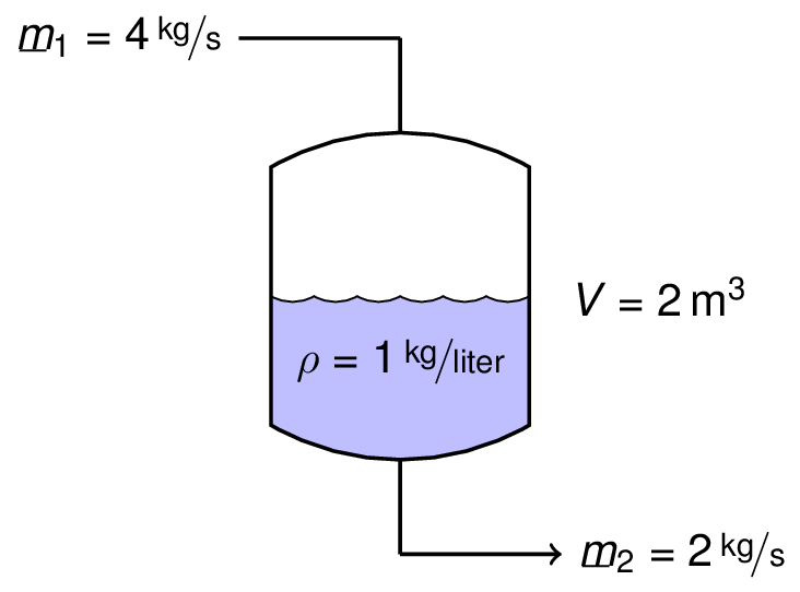 # ### Mass Balance
# Using our general principles for a mass balance
#
# $\frac{d(\rho V)}{dt} = \dot{m}_1 - \dot{m}_2$
#
# which can be simplified to
#
# $\frac{dV}{dt} = \frac{1}{\rho}\left(\dot{m}_1 - \dot{m}_2\right)$
#
# where the initial value is $V(0) = 1\,\mbox{m}^3$. This is a differential equation.
# ### Numerical Solution using `odeint`
# There are a number of numerical methods available for solving differential equations. Here we use [`odeint`](http://docs.scipy.org/doc/scipy/reference/generated/scipy.integrate.odeint.html) which is part of the [`scipy`](http://www.scipy.org/) package. `odeint` requires a function that returns the rate of accumulation in the tank as a function of the current volume and time.
# In[1]:
import numpy as np
import matplotlib.pyplot as plt
get_ipython().run_line_magic('matplotlib', 'inline')
from scipy.integrate import odeint
# In[2]:
# Flowrates in kg/sec
m1 = 4.0
m2 = 2.0
# Density in kg/m**3
rho = 1000.0
# Function to compute accumulation rate
def dV(V,t): return (m1 - m2)/rho;
# Next we import `odeint` from the `scipy.integrate` package, set up a grid of times at which we wish to find solution values, then call `odeint` to compute values for the solution starting with an initial condition of 1.0.
# In[3]:
t = np.linspace(0,1000)
V = odeint(dV,1.0,t)
# We finish by plotting the results of the integration and comparing to the capacity of the tank.
# In[4]:
plt.plot(t,V,'b',t,2*np.ones(len(t)),'r')
plt.xlabel('Time [sec]')
plt.ylabel('Volume [m**3]')
plt.legend(['Water Volume','Tank Capacity'],loc='upper left');
# This same approach can be used solve systems of differential equations. For an light-hearted (but very useful) example, check out [this solution](http://wiki.scipy.org/Cookbook/Zombie_Apocalypse_ODEINT) for the [Zombie Apocalypse](http://mysite.science.uottawa.ca/rsmith43/Zombies.pdf).
# ### Solving for the Time Required to Fill the Tank
# Now that we know how to solve the differential equation, next we create a function to compute the air volume of the tank at any given time.
# In[5]:
Vtank = 2.0
Vinitial = 1.0
def Vwater(t):
return odeint(dV,Vinitial,[0,t])[-1][0]
def Vair(t):
return Vtank - Vwater(t)
print("Air volume in the tank at t = 100 is {:4.2f} m**3.".format(Vair(100)))
# The next step is find the time at which `Vair(t)` returns a value of 0. This is [root finding](http://docs.scipy.org/doc/scipy/reference/tutorial/optimize.html#root-finding) which the function [`brentq`](http://docs.scipy.org/doc/scipy-0.13.0/reference/generated/scipy.optimize.brentq.html) will do for us.
# In[6]:
from scipy.optimize import brentq
t_full = brentq(Vair,0,1000)
print("The tank will be full at t = {:6.2f} seconds.".format(t_full))
# ## Exercise
# Suppose the tank was being used to protect against surges in water flow, and the inlet flowrate was a function of time where
#
# $\dot{m}_1 = 4 e^{-t/500}$
#
# * Will the tank overflow?
# * Assuming it doesn't overflow, how long would it take for the tank to return to its initial condition of being half full? To empty completely?
# * What will be the peak volume of water in the tank, and when will that occur?
# In[ ]:
#
# < [Ethylene Oxide Flowsheet](http://nbviewer.jupyter.org/github/jckantor/CBE20255/blob/master/notebooks/04.02-Ethylene-Oxide-Flowsheet.ipynb) | [Contents](toc.ipynb) | [Unsteady-State Material Balances](http://nbviewer.jupyter.org/github/jckantor/CBE20255/blob/master/notebooks/04.04-Unsteady-State-Material-Balances.ipynb) >
# ### Mass Balance
# Using our general principles for a mass balance
#
# $\frac{d(\rho V)}{dt} = \dot{m}_1 - \dot{m}_2$
#
# which can be simplified to
#
# $\frac{dV}{dt} = \frac{1}{\rho}\left(\dot{m}_1 - \dot{m}_2\right)$
#
# where the initial value is $V(0) = 1\,\mbox{m}^3$. This is a differential equation.
# ### Numerical Solution using `odeint`
# There are a number of numerical methods available for solving differential equations. Here we use [`odeint`](http://docs.scipy.org/doc/scipy/reference/generated/scipy.integrate.odeint.html) which is part of the [`scipy`](http://www.scipy.org/) package. `odeint` requires a function that returns the rate of accumulation in the tank as a function of the current volume and time.
# In[1]:
import numpy as np
import matplotlib.pyplot as plt
get_ipython().run_line_magic('matplotlib', 'inline')
from scipy.integrate import odeint
# In[2]:
# Flowrates in kg/sec
m1 = 4.0
m2 = 2.0
# Density in kg/m**3
rho = 1000.0
# Function to compute accumulation rate
def dV(V,t): return (m1 - m2)/rho;
# Next we import `odeint` from the `scipy.integrate` package, set up a grid of times at which we wish to find solution values, then call `odeint` to compute values for the solution starting with an initial condition of 1.0.
# In[3]:
t = np.linspace(0,1000)
V = odeint(dV,1.0,t)
# We finish by plotting the results of the integration and comparing to the capacity of the tank.
# In[4]:
plt.plot(t,V,'b',t,2*np.ones(len(t)),'r')
plt.xlabel('Time [sec]')
plt.ylabel('Volume [m**3]')
plt.legend(['Water Volume','Tank Capacity'],loc='upper left');
# This same approach can be used solve systems of differential equations. For an light-hearted (but very useful) example, check out [this solution](http://wiki.scipy.org/Cookbook/Zombie_Apocalypse_ODEINT) for the [Zombie Apocalypse](http://mysite.science.uottawa.ca/rsmith43/Zombies.pdf).
# ### Solving for the Time Required to Fill the Tank
# Now that we know how to solve the differential equation, next we create a function to compute the air volume of the tank at any given time.
# In[5]:
Vtank = 2.0
Vinitial = 1.0
def Vwater(t):
return odeint(dV,Vinitial,[0,t])[-1][0]
def Vair(t):
return Vtank - Vwater(t)
print("Air volume in the tank at t = 100 is {:4.2f} m**3.".format(Vair(100)))
# The next step is find the time at which `Vair(t)` returns a value of 0. This is [root finding](http://docs.scipy.org/doc/scipy/reference/tutorial/optimize.html#root-finding) which the function [`brentq`](http://docs.scipy.org/doc/scipy-0.13.0/reference/generated/scipy.optimize.brentq.html) will do for us.
# In[6]:
from scipy.optimize import brentq
t_full = brentq(Vair,0,1000)
print("The tank will be full at t = {:6.2f} seconds.".format(t_full))
# ## Exercise
# Suppose the tank was being used to protect against surges in water flow, and the inlet flowrate was a function of time where
#
# $\dot{m}_1 = 4 e^{-t/500}$
#
# * Will the tank overflow?
# * Assuming it doesn't overflow, how long would it take for the tank to return to its initial condition of being half full? To empty completely?
# * What will be the peak volume of water in the tank, and when will that occur?
# In[ ]:
#
# < [Ethylene Oxide Flowsheet](http://nbviewer.jupyter.org/github/jckantor/CBE20255/blob/master/notebooks/04.02-Ethylene-Oxide-Flowsheet.ipynb) | [Contents](toc.ipynb) | [Unsteady-State Material Balances](http://nbviewer.jupyter.org/github/jckantor/CBE20255/blob/master/notebooks/04.04-Unsteady-State-Material-Balances.ipynb) >