#!/usr/bin/env python
# coding: utf-8
#
# *This notebook contains course material from [CBE20255](https://jckantor.github.io/CBE20255)
# by Jeffrey Kantor (jeff at nd.edu); the content is available [on Github](https://github.com/jckantor/CBE20255.git).
# The text is released under the [CC-BY-NC-ND-4.0 license](https://creativecommons.org/licenses/by-nc-nd/4.0/legalcode),
# and code is released under the [MIT license](https://opensource.org/licenses/MIT).*
#
# < [Process Flows and Balances](http://nbviewer.jupyter.org/github/jckantor/CBE20255/blob/master/notebooks/03.00-Process-Flows-and-Balances.ipynb) | [Contents](toc.ipynb) | [CO2 Production by Automobiles](http://nbviewer.jupyter.org/github/jckantor/CBE20255/blob/master/notebooks/03.02-CO2-Production-by-Automobiles.ipynb) > # # Global CO2 Budget
# ## Summary
#
# This [Jupyter notebook](http://jupyter.org/notebook.html) provides an analysis of global CO2 emissions go by solving a mass balance.
# ## Problem Statement
#
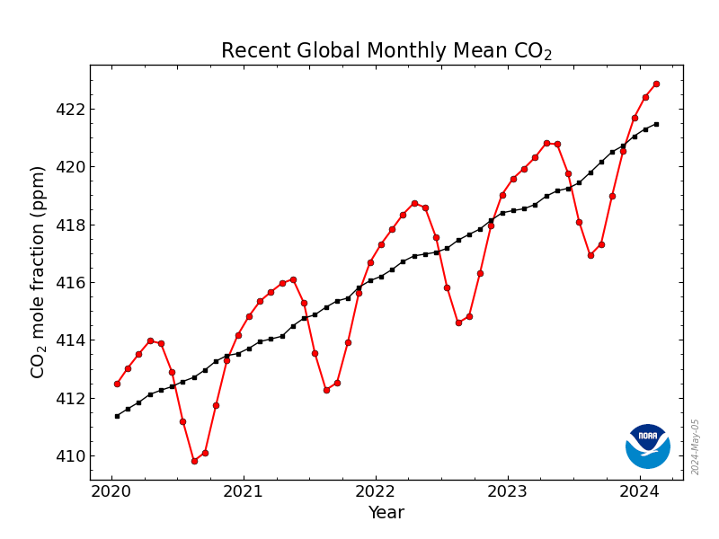
# The total global emissons of CO2 is estimated by the [Netherlands Environmental Assessment Agency](http://www.pbl.nl/en/publications/trends-in-global-co2-emissions-2013-report) to be 34.5 billion metric tons from all sources, including fossil fuels, cement production, and land use changes. [As measured by NOAA](http://www.esrl.noaa.gov/gmd/ccgg/trends/global.html), in recent years the atmospheric concentration of CO2 is increasing at an annual rate of about 2.4 ppmv (parts per million by volume).
#
#
# # Global CO2 Budget
# ## Summary
#
# This [Jupyter notebook](http://jupyter.org/notebook.html) provides an analysis of global CO2 emissions go by solving a mass balance.
# ## Problem Statement
#
# The total global emissons of CO2 is estimated by the [Netherlands Environmental Assessment Agency](http://www.pbl.nl/en/publications/trends-in-global-co2-emissions-2013-report) to be 34.5 billion metric tons from all sources, including fossil fuels, cement production, and land use changes. [As measured by NOAA](http://www.esrl.noaa.gov/gmd/ccgg/trends/global.html), in recent years the atmospheric concentration of CO2 is increasing at an annual rate of about 2.4 ppmv (parts per million by volume).
#
#  #
# Assuming these numbers are accurate and that the atmosphere is well mixed, what fraction of global CO2 emissions are being retained in the atmosphere?
# ## Solution
#
# This problem requires us to perform a material balance for CO2 in the atmosphere. We'll perform the using a 10 step approach outlined in the textbook.
# ### Step 1. Draw a diagram.
#
#
#
# Assuming these numbers are accurate and that the atmosphere is well mixed, what fraction of global CO2 emissions are being retained in the atmosphere?
# ## Solution
#
# This problem requires us to perform a material balance for CO2 in the atmosphere. We'll perform the using a 10 step approach outlined in the textbook.
# ### Step 1. Draw a diagram.
#
# 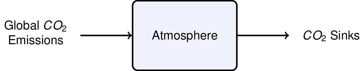 # ### Step 2. Define the system of interest.
#
# The system of interest is the global atmosphere which we assume is well mixed and of uniform composition.
# ### Step 3. Choose components and define stream variables.
#
# The chemical component to model is CO2. The stream variables are the mass flowrates of CO2 into and out of the atmosphere.
# ### Step 4. Convert all units to consistent units of mass or moles.
#
# This problem could be done on either a molar or mass basis. We'll arbitrarily choose to do this in mass units of kg/year. First we convert global emissions to kg/year.
# In[ ]:
get_ipython().run_line_magic('matplotlib', 'inline')
from numpy import *
# In[ ]:
mCO2_in = 34.5e9 # inflow, metric tonnes per year
mCO2_in = mCO2_in*1000 # inflow, kg per year
print("Global CO2 emissions = {:8.3g} kg/yr".format(mCO2_in))
# The rate of accumulation is given as ppm by volume per year. For ideal gases, volume fraction is equivalent to mole fraction. We need to convert the mole fraction, which is the ratio of kg-moles of CO2 to kg-moles of air, to mass fraction which has units of kg of CO2 to kg of air per year.
# In[ ]:
nCO2_accum = 2.4e-6 # accumulation, kg-mol CO2/kg-mol air/yr
mwAir = 28.97 # kg air/kg-mol air
mwCO2 = 44.01 # kg CO2/kg-mol CO2
wCO2_accum = nCO2_accum*mwCO2/mwAir # kg CO2/kg air/yr
print("Accumulation Rate of CO2 = {:8.3g} kg CO2/kg air".format(wCO2_accum))
# ### Step 5. Define a basis.
#
# The basis for the calculation are flows and change in one year. No additional work is required.
# ### Step 6. Define system variables.
#
# The system variable is the rate of accumulation of CO2 in kg CO2/year. We need to convert from change in concentration per year to change in total mass per year. The first step is to estimate the total mass of air.
# In[ ]:
# Earth Radius in meters
R = 6371000 # m
# Earth Area in square meters
A = 4*pi*R**2 # m**2
# Mass of the atmosphere in kg
g = 9.81 # N/kg
P = 101325 # N/m**2
mAir = A*P/g # kg
print("Estimated mass of the atmosphere = {:8.3g} kg".format(mAir))
# To get the rate of change of total CO2, multiply the total mass of by the rate of change of mass fraction of CO2.
# In[ ]:
mCO2_accum = wCO2_accum*mAir # kg CO2/year
print("Change in CO2 = {:8.3g} kg CO2/year".format(mCO2_accum))
# ### Step 7. List specifications
#
# The inflow and rate of change of CO2 are specified, and calculated above.
# ### Step 8. Write material balance equations for each species.
#
# $$\mbox{Accumulation} = \mbox{Inflow} - \mbox{Outflow} + \underbrace{\mbox{Generation}}_{=0} - \underbrace{\mbox{Consumption}}_{=0}$$
# ### Step 9. Solve material balance equations.
#
# $$\mbox{Outflow} = \mbox{Inflow} - \mbox{Accumulation}$$
# In[ ]:
mCO2_out = mCO2_in - mCO2_accum
print("Global CO2 outflow = {:8.3g} kg CO2/yr".format(mCO2_out))
#
# ### Step 10. Check your work.
#
# Fraction retained in the atmosphere
# In[ ]:
fCO2 = mCO2_accum/mCO2_in
print("Fraction of CO2 retained in the atmosphere = {:<.2g} ".format(fCO2))
# In[ ]:
#
# < [Process Flows and Balances](http://nbviewer.jupyter.org/github/jckantor/CBE20255/blob/master/notebooks/03.00-Process-Flows-and-Balances.ipynb) | [Contents](toc.ipynb) | [CO2 Production by Automobiles](http://nbviewer.jupyter.org/github/jckantor/CBE20255/blob/master/notebooks/03.02-CO2-Production-by-Automobiles.ipynb) >
# ### Step 2. Define the system of interest.
#
# The system of interest is the global atmosphere which we assume is well mixed and of uniform composition.
# ### Step 3. Choose components and define stream variables.
#
# The chemical component to model is CO2. The stream variables are the mass flowrates of CO2 into and out of the atmosphere.
# ### Step 4. Convert all units to consistent units of mass or moles.
#
# This problem could be done on either a molar or mass basis. We'll arbitrarily choose to do this in mass units of kg/year. First we convert global emissions to kg/year.
# In[ ]:
get_ipython().run_line_magic('matplotlib', 'inline')
from numpy import *
# In[ ]:
mCO2_in = 34.5e9 # inflow, metric tonnes per year
mCO2_in = mCO2_in*1000 # inflow, kg per year
print("Global CO2 emissions = {:8.3g} kg/yr".format(mCO2_in))
# The rate of accumulation is given as ppm by volume per year. For ideal gases, volume fraction is equivalent to mole fraction. We need to convert the mole fraction, which is the ratio of kg-moles of CO2 to kg-moles of air, to mass fraction which has units of kg of CO2 to kg of air per year.
# In[ ]:
nCO2_accum = 2.4e-6 # accumulation, kg-mol CO2/kg-mol air/yr
mwAir = 28.97 # kg air/kg-mol air
mwCO2 = 44.01 # kg CO2/kg-mol CO2
wCO2_accum = nCO2_accum*mwCO2/mwAir # kg CO2/kg air/yr
print("Accumulation Rate of CO2 = {:8.3g} kg CO2/kg air".format(wCO2_accum))
# ### Step 5. Define a basis.
#
# The basis for the calculation are flows and change in one year. No additional work is required.
# ### Step 6. Define system variables.
#
# The system variable is the rate of accumulation of CO2 in kg CO2/year. We need to convert from change in concentration per year to change in total mass per year. The first step is to estimate the total mass of air.
# In[ ]:
# Earth Radius in meters
R = 6371000 # m
# Earth Area in square meters
A = 4*pi*R**2 # m**2
# Mass of the atmosphere in kg
g = 9.81 # N/kg
P = 101325 # N/m**2
mAir = A*P/g # kg
print("Estimated mass of the atmosphere = {:8.3g} kg".format(mAir))
# To get the rate of change of total CO2, multiply the total mass of by the rate of change of mass fraction of CO2.
# In[ ]:
mCO2_accum = wCO2_accum*mAir # kg CO2/year
print("Change in CO2 = {:8.3g} kg CO2/year".format(mCO2_accum))
# ### Step 7. List specifications
#
# The inflow and rate of change of CO2 are specified, and calculated above.
# ### Step 8. Write material balance equations for each species.
#
# $$\mbox{Accumulation} = \mbox{Inflow} - \mbox{Outflow} + \underbrace{\mbox{Generation}}_{=0} - \underbrace{\mbox{Consumption}}_{=0}$$
# ### Step 9. Solve material balance equations.
#
# $$\mbox{Outflow} = \mbox{Inflow} - \mbox{Accumulation}$$
# In[ ]:
mCO2_out = mCO2_in - mCO2_accum
print("Global CO2 outflow = {:8.3g} kg CO2/yr".format(mCO2_out))
#
# ### Step 10. Check your work.
#
# Fraction retained in the atmosphere
# In[ ]:
fCO2 = mCO2_accum/mCO2_in
print("Fraction of CO2 retained in the atmosphere = {:<.2g} ".format(fCO2))
# In[ ]:
#
# < [Process Flows and Balances](http://nbviewer.jupyter.org/github/jckantor/CBE20255/blob/master/notebooks/03.00-Process-Flows-and-Balances.ipynb) | [Contents](toc.ipynb) | [CO2 Production by Automobiles](http://nbviewer.jupyter.org/github/jckantor/CBE20255/blob/master/notebooks/03.02-CO2-Production-by-Automobiles.ipynb) >