#!/usr/bin/env python
# coding: utf-8
# Table of Contents
#
#  # In[2]:
import pandas as pd
import numpy as np # necessity as pandas is built on np
from IPython.display import Image # to display images
# The Pandas library is built on NumPy and provides easy-to-use data structures and data analysis tools for the Python programming language.
#
# Refer to these cheatsheets:
# https://s3.amazonaws.com/assets.datacamp.com/blog_assets/PandasPythonForDataScience+(1).pdf
# https://s3.amazonaws.com/assets.datacamp.com/blog_assets/Python_Pandas_Cheat_Sheet_2.pdf
# ### Input/Output
# Different types of data can be loaded in pandas dataframe. Pandas dataframe is like looks spreadsheet table (just a rough analogy)
# * **Most common input types**
# * `pd.read_csv`
# * `pd.read_excel/ pd.ExcelFile`
# * `pd.read_feather` (feather format is used to reduce memory load in df as data is saved in binary form)
# * `pd.read_json`
# * `pd.read_html`
# * `pd.read_pickle` (can also infer if pickled object is zipped using infer=)
#
# * **Output types have format `to_xxx` similar to input formats**
# ### Pandas data structures
# ** Pandas data strctures include `series` and `dataframe` **
# **Series**: A one-dimensional labeled array a capable of holding any data type
# In[18]:
Image('../images/series.png', width=500) # not pandas, just showing example series
# In[22]:
# index will set the index for further reference
# data can be passed as list
s = pd.Series([3, -5, 7, 4], index=['a', 'b', 'c', 'd'])
# In[21]:
s
# **Can be indexed using both index name or number.**
# number: --> filter indexes after value of number
# :number --> filter indexes before value of number
# In[42]:
s[1:]
# In[46]:
s['a']
# In[47]:
s[:'c']
# In[50]:
s.index
# In[37]:
# series using dictionary
s2 = pd.Series({'a':3, 'b': -1, 'c': 12}); s2
# In[38]:
s2['b']
# **Dataframe**: A two-dimensional labeled data structure with columns of potentially different types. It is similar to excel table.
#
# Can make data frame using dictionary, list of list
# In[25]:
Image('../images/df.png', width=500)
# In[288]:
data = {'Country': ['Belgium', 'India', 'Brazil'],
'Capital': ['Brussels', 'New Delhi', 'Brasília'],
'Population': [11190846, 1303171035, 207847528]}
# In[289]:
df_sample = pd.DataFrame(data,
columns=['Country', 'Capital', 'Population'])
# In[290]:
df_sample
# ### Common dataframe functionality
# Using famous `titanic data` for analysis and exploration.
# https://www.kaggle.com/c/titanic/data
#
# In[2]:
import pandas as pd
import numpy as np # necessity as pandas is built on np
from IPython.display import Image # to display images
# The Pandas library is built on NumPy and provides easy-to-use data structures and data analysis tools for the Python programming language.
#
# Refer to these cheatsheets:
# https://s3.amazonaws.com/assets.datacamp.com/blog_assets/PandasPythonForDataScience+(1).pdf
# https://s3.amazonaws.com/assets.datacamp.com/blog_assets/Python_Pandas_Cheat_Sheet_2.pdf
# ### Input/Output
# Different types of data can be loaded in pandas dataframe. Pandas dataframe is like looks spreadsheet table (just a rough analogy)
# * **Most common input types**
# * `pd.read_csv`
# * `pd.read_excel/ pd.ExcelFile`
# * `pd.read_feather` (feather format is used to reduce memory load in df as data is saved in binary form)
# * `pd.read_json`
# * `pd.read_html`
# * `pd.read_pickle` (can also infer if pickled object is zipped using infer=)
#
# * **Output types have format `to_xxx` similar to input formats**
# ### Pandas data structures
# ** Pandas data strctures include `series` and `dataframe` **
# **Series**: A one-dimensional labeled array a capable of holding any data type
# In[18]:
Image('../images/series.png', width=500) # not pandas, just showing example series
# In[22]:
# index will set the index for further reference
# data can be passed as list
s = pd.Series([3, -5, 7, 4], index=['a', 'b', 'c', 'd'])
# In[21]:
s
# **Can be indexed using both index name or number.**
# number: --> filter indexes after value of number
# :number --> filter indexes before value of number
# In[42]:
s[1:]
# In[46]:
s['a']
# In[47]:
s[:'c']
# In[50]:
s.index
# In[37]:
# series using dictionary
s2 = pd.Series({'a':3, 'b': -1, 'c': 12}); s2
# In[38]:
s2['b']
# **Dataframe**: A two-dimensional labeled data structure with columns of potentially different types. It is similar to excel table.
#
# Can make data frame using dictionary, list of list
# In[25]:
Image('../images/df.png', width=500)
# In[288]:
data = {'Country': ['Belgium', 'India', 'Brazil'],
'Capital': ['Brussels', 'New Delhi', 'Brasília'],
'Population': [11190846, 1303171035, 207847528]}
# In[289]:
df_sample = pd.DataFrame(data,
columns=['Country', 'Capital', 'Population'])
# In[290]:
df_sample
# ### Common dataframe functionality
# Using famous `titanic data` for analysis and exploration.
# https://www.kaggle.com/c/titanic/data
#  # * **Common things to do when we get data in a dataframe (examples shown below):**
# * see dataframe shape (number of rows, number of columns) using `df.shape`
# * see top 5 rows using `pd.head()`
# * check datatype of each column using `pd.dtypes`
# * check column names using `pd.columns`
# * count unique values of each column to see cardinality levels using `pd.nunique()`
# * number of non null in each column, memory usage of df, datatype (especially for large df) using `pd.info()`
#
#
# In[3]:
df = pd.read_csv('../data/train.csv') # read csv file
# In[33]:
df.shape
# In[8]:
df.head() # see top 5 rows of data
# In[26]:
df.dtypes # see datatype of each variable
# In[27]:
df.columns # column names
# In[32]:
df.nunique() # unique value for each variable
# In[34]:
df.info() # not null part is very useful to see how many nulls are there in data
# ### Advanced Indexing
# #### `iloc`
# Select based on integer location (**that's why i**). Can select single or multiple
# In[56]:
df.iloc[0, 4] # 0 row, 4 column
# In[58]:
df.iloc[1:4, 2:6] # indexes are maintained. Can reset_index() to start index from 0
# #### `loc`
# Select based on label name of column (can select single or multiple)
# In[63]:
df.loc[1:2,'Name':"Age"] # here row indexes are numbers but column indexes are name of columns
# In[4]:
df.loc[2,['Name',"Age"]] # here row indexes are numbers.
# #### `ix`
# ix has been deprecated in latest pandas library. It was used to select by label or position. But we can always use `loc` to select with labels and `iloc` to select with integers/position
# #### `Boolean indexing`
# Returns rows where the stated condition returns true
#
# * or -> condition 1 `|` condition 2 (`or` also works but throws ambiguity error for multiple conditions)
# * and -> condition 1 `&` condition 2 (`and` also works but throws ambiguity error for multiple conditions
# * not -> `~` (not condition)
# * equal -> `==` Satisfying condition
# * `any()` -> columns/rows with any value matching condition
# * `all()` > columns/rows with all values matching some condition
# In[31]:
# select rows with either sex as female or Pclass as 1
df[(df.Sex == 'female') | (df.iloc[:,2] == 1) ].iloc[:3] # () are important
# In[63]:
# first 3 rows of gives all columns which have all string values or all int > 1 values
df.loc[:,(df > 1).all()][:3]
# In[65]:
# first 3 rows of all columns which have all not null values
df.loc[:,(df.notnull().all() )][:3]
# In[67]:
# first 3 rows of all columns which have atleast 1 null value
df.loc[:, df.isnull().any()][:3]
# In[33]:
df[(df.iloc[:,2] == 1) & (df.Sex == 'female')].shape
# In[39]:
# fraction of males with Age > 25, df.shape[0] -> number of rows
sum((df.Age > 25) & (df.Sex == 'male'))/df.shape[0]
# In[50]:
# number of people who survived and were not in class 3
sum((df.Survived != 0) & (~(df.Pclass == 3)) )
# #### `querying`
# Query columns (filter rows) of dataframe with boolean expression (Filter based on condition)
# In[75]:
# filter all rows which have Age > Passenger ID
df.query('Age > PassengerId')
# `filter`
#
# Filter dataframe on column names or row names (labels) by regrex or just item names
# In[3]:
# filter only sex and age columns (first 2 rows)
df.filter(items=['Age', 'Sex'])[:2]
# In[6]:
# filter only 0 and 5 row index
df.filter(items=[0,5], axis=0)
# In[8]:
# first 2 rows of column names ending with "ed" (think of past tense)
df.filter(like = 'ed', axis=1)[:2]
# In[20]:
# Can use same thing as above using regex also
df.filter(regex='ed$', axis=1)[:2]
# #### `isin`
#
# Filter rows of column based on list of multiple values
# In[28]:
df[df.Pclass.isin([0,1])].head()
# ### Setting/ Resetting Index
# Setting and resetting index are important when we merge/groupby 2 dataframe and want to do further analysis on new dataframe. A dataframe with repeated indexes can cause problems in filtering. Apart from this we cvan set a column into index which makes merging much faster
# #### `set_index()`
# Set any column you want as index of df
# In[76]:
# setting
df.set_index('Ticket')[:2]
# In[77]:
# can set multiple columns as index also. Just pass them in list
# Setting Ticket and Name as index
df.set_index(['Ticket', 'Name'])[:2]
# In[90]:
# can see what are values of index.
# checking index of 1st row
df.set_index(['Ticket', 'Name']).index[0]
# #### `reset_index()`
# Can reset index back to 0....nrows-1
# In[91]:
df_index = df.set_index(['Ticket', 'Name'])
# In[92]:
df_index[:2]
# In[93]:
df_index.reset_index()[:2]
# In above case, index is back to 0,1...
# #### `rename()`
# Renaming column names or row indexes of dataframe. Default is index
# In[94]:
df.rename(columns={'Name': 'Whats_name', 'Fare':'Price'})[:2]
# In[96]:
# can use some mapper function also. default axis='index' (0)
df.rename(mapper=str.lower, axis='columns')[:2]
# ### Duplicated data
# #### `unique()`
# Number of unique values in a column of df (Use nunique() for count of unique in each column)
# In[98]:
df.Sex.unique()
# #### `duplicated()`
# Check duplicated in column. Returns True/False
# In[102]:
sum(df.PassengerId.duplicated()) # there are no duplicate passegerid. good thing to check
# In[115]:
# can check duplicates in index also.
# useful if doubtful about duplicates in index doing bad things
sum(df.index.duplicated())
# #### `drop_duplicates`
# Drop rows which have duplicates
# In[106]:
# can help in getting unique combination of multiple columns
# unique() dosn't work in this case
df.loc[:,['Sex', 'Embarked']].drop_duplicates()
# ### Grouping data
# Group by some column/columns, then we can aggregate to get mean, count, sum or custom function based on the group
# #### `groupby`
# In[123]:
# group by sex then count.
# returns count in each column. difference in some cases because of nulls in those columns
# can do iloc[:,0] to only get first column
df.groupby(by = ['Sex']).count()
# In[125]:
# can use multiple conditions
# group by sex and survived -> mean of age
df.groupby(by = ['Sex', 'Survived']).mean().loc[:,'Age']
# In[145]:
# can group by indexes also by using levels=
# useful when we have multindexes
# can use agg function with lambda func
df_index = df.set_index(['Sex', 'Pclass'])
df_index.groupby(level=[0,1]).agg({'Fare': lambda x: sum(x)/len(x), # this is also just mean actually
'Age' : np.mean})
# Interesting! Ticket price of 1st class female is approximately double of 1st class male
# #### `transform`
# Can apply such functions for all columns also using transform which transforms all rows
#
# In[153]:
# shape of below code is same as original df
df_index.groupby(level=[0,1]).transform(lambda x: sum(x)/len(x)).head()
# ### Handling missing data
# #### `dropna`
# Drop rows with na
# In[156]:
# how=any -> row with any column = NA
df.dropna(axis=0, how='any').shape
# In[159]:
# how=any -> row with all columns = NA
df.dropna(axis=0, how='all').shape
# In[167]:
# drops column which have any row of NA
[set(df.columns) - set(df.dropna(axis=1, how='any').columns)]
# Three columns have been removed
# #### `fillna`
# In[173]:
# replace with mean of that column
# can put any specific value also
# would not work for columns with string type like Cabin
df.fillna(np.mean)[:1]
# ### Combining Data
#
# * **Common things to do when we get data in a dataframe (examples shown below):**
# * see dataframe shape (number of rows, number of columns) using `df.shape`
# * see top 5 rows using `pd.head()`
# * check datatype of each column using `pd.dtypes`
# * check column names using `pd.columns`
# * count unique values of each column to see cardinality levels using `pd.nunique()`
# * number of non null in each column, memory usage of df, datatype (especially for large df) using `pd.info()`
#
#
# In[3]:
df = pd.read_csv('../data/train.csv') # read csv file
# In[33]:
df.shape
# In[8]:
df.head() # see top 5 rows of data
# In[26]:
df.dtypes # see datatype of each variable
# In[27]:
df.columns # column names
# In[32]:
df.nunique() # unique value for each variable
# In[34]:
df.info() # not null part is very useful to see how many nulls are there in data
# ### Advanced Indexing
# #### `iloc`
# Select based on integer location (**that's why i**). Can select single or multiple
# In[56]:
df.iloc[0, 4] # 0 row, 4 column
# In[58]:
df.iloc[1:4, 2:6] # indexes are maintained. Can reset_index() to start index from 0
# #### `loc`
# Select based on label name of column (can select single or multiple)
# In[63]:
df.loc[1:2,'Name':"Age"] # here row indexes are numbers but column indexes are name of columns
# In[4]:
df.loc[2,['Name',"Age"]] # here row indexes are numbers.
# #### `ix`
# ix has been deprecated in latest pandas library. It was used to select by label or position. But we can always use `loc` to select with labels and `iloc` to select with integers/position
# #### `Boolean indexing`
# Returns rows where the stated condition returns true
#
# * or -> condition 1 `|` condition 2 (`or` also works but throws ambiguity error for multiple conditions)
# * and -> condition 1 `&` condition 2 (`and` also works but throws ambiguity error for multiple conditions
# * not -> `~` (not condition)
# * equal -> `==` Satisfying condition
# * `any()` -> columns/rows with any value matching condition
# * `all()` > columns/rows with all values matching some condition
# In[31]:
# select rows with either sex as female or Pclass as 1
df[(df.Sex == 'female') | (df.iloc[:,2] == 1) ].iloc[:3] # () are important
# In[63]:
# first 3 rows of gives all columns which have all string values or all int > 1 values
df.loc[:,(df > 1).all()][:3]
# In[65]:
# first 3 rows of all columns which have all not null values
df.loc[:,(df.notnull().all() )][:3]
# In[67]:
# first 3 rows of all columns which have atleast 1 null value
df.loc[:, df.isnull().any()][:3]
# In[33]:
df[(df.iloc[:,2] == 1) & (df.Sex == 'female')].shape
# In[39]:
# fraction of males with Age > 25, df.shape[0] -> number of rows
sum((df.Age > 25) & (df.Sex == 'male'))/df.shape[0]
# In[50]:
# number of people who survived and were not in class 3
sum((df.Survived != 0) & (~(df.Pclass == 3)) )
# #### `querying`
# Query columns (filter rows) of dataframe with boolean expression (Filter based on condition)
# In[75]:
# filter all rows which have Age > Passenger ID
df.query('Age > PassengerId')
# `filter`
#
# Filter dataframe on column names or row names (labels) by regrex or just item names
# In[3]:
# filter only sex and age columns (first 2 rows)
df.filter(items=['Age', 'Sex'])[:2]
# In[6]:
# filter only 0 and 5 row index
df.filter(items=[0,5], axis=0)
# In[8]:
# first 2 rows of column names ending with "ed" (think of past tense)
df.filter(like = 'ed', axis=1)[:2]
# In[20]:
# Can use same thing as above using regex also
df.filter(regex='ed$', axis=1)[:2]
# #### `isin`
#
# Filter rows of column based on list of multiple values
# In[28]:
df[df.Pclass.isin([0,1])].head()
# ### Setting/ Resetting Index
# Setting and resetting index are important when we merge/groupby 2 dataframe and want to do further analysis on new dataframe. A dataframe with repeated indexes can cause problems in filtering. Apart from this we cvan set a column into index which makes merging much faster
# #### `set_index()`
# Set any column you want as index of df
# In[76]:
# setting
df.set_index('Ticket')[:2]
# In[77]:
# can set multiple columns as index also. Just pass them in list
# Setting Ticket and Name as index
df.set_index(['Ticket', 'Name'])[:2]
# In[90]:
# can see what are values of index.
# checking index of 1st row
df.set_index(['Ticket', 'Name']).index[0]
# #### `reset_index()`
# Can reset index back to 0....nrows-1
# In[91]:
df_index = df.set_index(['Ticket', 'Name'])
# In[92]:
df_index[:2]
# In[93]:
df_index.reset_index()[:2]
# In above case, index is back to 0,1...
# #### `rename()`
# Renaming column names or row indexes of dataframe. Default is index
# In[94]:
df.rename(columns={'Name': 'Whats_name', 'Fare':'Price'})[:2]
# In[96]:
# can use some mapper function also. default axis='index' (0)
df.rename(mapper=str.lower, axis='columns')[:2]
# ### Duplicated data
# #### `unique()`
# Number of unique values in a column of df (Use nunique() for count of unique in each column)
# In[98]:
df.Sex.unique()
# #### `duplicated()`
# Check duplicated in column. Returns True/False
# In[102]:
sum(df.PassengerId.duplicated()) # there are no duplicate passegerid. good thing to check
# In[115]:
# can check duplicates in index also.
# useful if doubtful about duplicates in index doing bad things
sum(df.index.duplicated())
# #### `drop_duplicates`
# Drop rows which have duplicates
# In[106]:
# can help in getting unique combination of multiple columns
# unique() dosn't work in this case
df.loc[:,['Sex', 'Embarked']].drop_duplicates()
# ### Grouping data
# Group by some column/columns, then we can aggregate to get mean, count, sum or custom function based on the group
# #### `groupby`
# In[123]:
# group by sex then count.
# returns count in each column. difference in some cases because of nulls in those columns
# can do iloc[:,0] to only get first column
df.groupby(by = ['Sex']).count()
# In[125]:
# can use multiple conditions
# group by sex and survived -> mean of age
df.groupby(by = ['Sex', 'Survived']).mean().loc[:,'Age']
# In[145]:
# can group by indexes also by using levels=
# useful when we have multindexes
# can use agg function with lambda func
df_index = df.set_index(['Sex', 'Pclass'])
df_index.groupby(level=[0,1]).agg({'Fare': lambda x: sum(x)/len(x), # this is also just mean actually
'Age' : np.mean})
# Interesting! Ticket price of 1st class female is approximately double of 1st class male
# #### `transform`
# Can apply such functions for all columns also using transform which transforms all rows
#
# In[153]:
# shape of below code is same as original df
df_index.groupby(level=[0,1]).transform(lambda x: sum(x)/len(x)).head()
# ### Handling missing data
# #### `dropna`
# Drop rows with na
# In[156]:
# how=any -> row with any column = NA
df.dropna(axis=0, how='any').shape
# In[159]:
# how=any -> row with all columns = NA
df.dropna(axis=0, how='all').shape
# In[167]:
# drops column which have any row of NA
[set(df.columns) - set(df.dropna(axis=1, how='any').columns)]
# Three columns have been removed
# #### `fillna`
# In[173]:
# replace with mean of that column
# can put any specific value also
# would not work for columns with string type like Cabin
df.fillna(np.mean)[:1]
# ### Combining Data
# 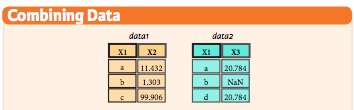 # #### `merge` / `join`
#
# * **how** = 'left', 'right', 'outer', 'inner'
# * **on**
#
# In[182]:
data1 = pd.DataFrame({'x1': list('abc'), 'x2': [11.432, 1.303, 99.906]})
# In[197]:
data2 = pd.DataFrame({'x1': list('abd'), 'x3': [20.784, np.NaN, 20.784]})
# In[183]:
data1
# In[198]:
data2
# In[199]:
# inner join when both table have that key (like sql)
data1.merge(data2, how='inner', on='x1')
# In[200]:
# outer joins on all keys in both df and creates NA
data1.merge(data2, how='outer', on='x1')
# can also use `join` but `merge` is faster. just use merge
# In[202]:
# if columns overlap, have to specify suffix as it makes for all
data1.join(data2, on='x1', how='left', lsuffix='L')
# #### `concatenate`
# In[223]:
# join over axis=0, i.e rows combine
# also adds all columns with na
pd.concat([data1, data2], axis=0)
# Notice that it has index duplicates as it maintain original df index
# Can use `ignore_index=True` to make index start from 0
# In[211]:
pd.concat([data1, data2], axis=0, ignore_index=True)
# In[217]:
data2.loc[3] = ['g', 500] # adding new row
data2
# In[228]:
# join over axis=1, i.e columns combine
pd.concat([data1, data2], axis=1)
# ### Date formatting
#
# * `to_datetime()` -> convert whatever format argument to datetime (obviously that can be parsed to datetime)
# * `date_range()` -> generates datetime data
# * `Datetimeindex` -> datetypeindex data
# In[246]:
pd.to_datetime('2018-2-19')
# In[250]:
# gives datetimeindex format
pd.date_range('2018-4-18', periods=6, freq='d')
# In[235]:
data1['date'] = pd.date_range('2018-4-18', periods=3, freq='d')
# In[236]:
data1
# In[248]:
data1.date
# In[247]:
pd.DatetimeIndex(data1.date)
# ### Reshaping data
# #### `pivot` -> reshape data
# Ever used pivot table in excel? It's same.
# In[252]:
# index = new index, columns = new_columns, values = values to put
df.pivot(index='Sex', columns = 'PassengerId', values = 'Age')
# In above case, use of pivot doesn't make sense but this is just an example
# #### `stack`
#
# Convert whole df into 1 long format
# In[258]:
df.stack()
# You won't generally use it. I have never come across its use over my experience with python
# ### Iteration
# To get column/row indexes, series pair.
#
# * `iteritems()` for column-index, series
# * `iterrows()` for row-index, series
# In[286]:
list(df.Sex.iteritems())[:5]
# In[285]:
list(df.iterrows())[0]
# ### Apply functions
#
# * `apply` -> apply function over df
# * `apply_map` -> apply function elementwise (for each series of df. think of column wise)
# In[338]:
# function squares when type(x) = float, cubes when type(x) = int, return same when other
f = lambda x: x**2 if type(x) == float else x**3 if type(x) == int else x
# In[335]:
# whole series is passed
df.Fare.apply(f)[:3]
# In[339]:
# elements are passed
df.applymap(f)[:3]
# ### Working with text data
# What all can we do when we have string datatype in pandas dataframe/series ?
# #### `str`
#
# Working with string format in pandas series/df
#
# We can do:
# * `str.upper()/lower()` to convert string into upper or lower case
# * `str.len()` to find the length of sting
# * `str.strip()/lstrip()/rstrip()` to strip spaces
# * `str.replace()` to replace anything from string
# * `str.split()` to split words of string or using some other delimiter
# * `str.get()` to access elements in slit list
# * `str.resplit()` spit in reverse order of string based on some delimiter
# * `str.extract()` extract specific thing from string. alphabet or number
#
# Let's see how to use all that in pandas series. Keep in mind pandas DataFrame has no attribute called `str` and works on Series object only. So, grab column of df, then apply `str`
#
# In[10]:
# converts all rows into lower
df.Name.str.lower().head()
# In[16]:
# converts all rows into upper
df.Sex.str.upper().head()
# In[17]:
# counts all the characters including spaces
df.Name.str.len().head()
# In[46]:
# splits strings in each row over whitespaces ()
# expand=True : expand columns
# pat = regex to split on
df.Name.str.split(pat=',',expand=True).head().rename(columns={0:'First_Name', 1: 'Last_Name'})
# In[42]:
# splits strings in each row over whitespaces ()
# expand=False : doesn't expand columns
# pat = regex to split on
df.Name.str.split(expand=False).head()
# In[49]:
# replace Mr. with empty space
df.Name.str.replace('Mr.', '').head()
# In[71]:
# get() is used to get particular row of split
df.Name.str.split().get(1)
# In[17]:
df.Name[:10]
# In[28]:
# Extract just last name
df.Name.str.extract('(?P[a-zA-Z]+)', expand=True).head()
# ### End
# #### `merge` / `join`
#
# * **how** = 'left', 'right', 'outer', 'inner'
# * **on**
#
# In[182]:
data1 = pd.DataFrame({'x1': list('abc'), 'x2': [11.432, 1.303, 99.906]})
# In[197]:
data2 = pd.DataFrame({'x1': list('abd'), 'x3': [20.784, np.NaN, 20.784]})
# In[183]:
data1
# In[198]:
data2
# In[199]:
# inner join when both table have that key (like sql)
data1.merge(data2, how='inner', on='x1')
# In[200]:
# outer joins on all keys in both df and creates NA
data1.merge(data2, how='outer', on='x1')
# can also use `join` but `merge` is faster. just use merge
# In[202]:
# if columns overlap, have to specify suffix as it makes for all
data1.join(data2, on='x1', how='left', lsuffix='L')
# #### `concatenate`
# In[223]:
# join over axis=0, i.e rows combine
# also adds all columns with na
pd.concat([data1, data2], axis=0)
# Notice that it has index duplicates as it maintain original df index
# Can use `ignore_index=True` to make index start from 0
# In[211]:
pd.concat([data1, data2], axis=0, ignore_index=True)
# In[217]:
data2.loc[3] = ['g', 500] # adding new row
data2
# In[228]:
# join over axis=1, i.e columns combine
pd.concat([data1, data2], axis=1)
# ### Date formatting
#
# * `to_datetime()` -> convert whatever format argument to datetime (obviously that can be parsed to datetime)
# * `date_range()` -> generates datetime data
# * `Datetimeindex` -> datetypeindex data
# In[246]:
pd.to_datetime('2018-2-19')
# In[250]:
# gives datetimeindex format
pd.date_range('2018-4-18', periods=6, freq='d')
# In[235]:
data1['date'] = pd.date_range('2018-4-18', periods=3, freq='d')
# In[236]:
data1
# In[248]:
data1.date
# In[247]:
pd.DatetimeIndex(data1.date)
# ### Reshaping data
# #### `pivot` -> reshape data
# Ever used pivot table in excel? It's same.
# In[252]:
# index = new index, columns = new_columns, values = values to put
df.pivot(index='Sex', columns = 'PassengerId', values = 'Age')
# In above case, use of pivot doesn't make sense but this is just an example
# #### `stack`
#
# Convert whole df into 1 long format
# In[258]:
df.stack()
# You won't generally use it. I have never come across its use over my experience with python
# ### Iteration
# To get column/row indexes, series pair.
#
# * `iteritems()` for column-index, series
# * `iterrows()` for row-index, series
# In[286]:
list(df.Sex.iteritems())[:5]
# In[285]:
list(df.iterrows())[0]
# ### Apply functions
#
# * `apply` -> apply function over df
# * `apply_map` -> apply function elementwise (for each series of df. think of column wise)
# In[338]:
# function squares when type(x) = float, cubes when type(x) = int, return same when other
f = lambda x: x**2 if type(x) == float else x**3 if type(x) == int else x
# In[335]:
# whole series is passed
df.Fare.apply(f)[:3]
# In[339]:
# elements are passed
df.applymap(f)[:3]
# ### Working with text data
# What all can we do when we have string datatype in pandas dataframe/series ?
# #### `str`
#
# Working with string format in pandas series/df
#
# We can do:
# * `str.upper()/lower()` to convert string into upper or lower case
# * `str.len()` to find the length of sting
# * `str.strip()/lstrip()/rstrip()` to strip spaces
# * `str.replace()` to replace anything from string
# * `str.split()` to split words of string or using some other delimiter
# * `str.get()` to access elements in slit list
# * `str.resplit()` spit in reverse order of string based on some delimiter
# * `str.extract()` extract specific thing from string. alphabet or number
#
# Let's see how to use all that in pandas series. Keep in mind pandas DataFrame has no attribute called `str` and works on Series object only. So, grab column of df, then apply `str`
#
# In[10]:
# converts all rows into lower
df.Name.str.lower().head()
# In[16]:
# converts all rows into upper
df.Sex.str.upper().head()
# In[17]:
# counts all the characters including spaces
df.Name.str.len().head()
# In[46]:
# splits strings in each row over whitespaces ()
# expand=True : expand columns
# pat = regex to split on
df.Name.str.split(pat=',',expand=True).head().rename(columns={0:'First_Name', 1: 'Last_Name'})
# In[42]:
# splits strings in each row over whitespaces ()
# expand=False : doesn't expand columns
# pat = regex to split on
df.Name.str.split(expand=False).head()
# In[49]:
# replace Mr. with empty space
df.Name.str.replace('Mr.', '').head()
# In[71]:
# get() is used to get particular row of split
df.Name.str.split().get(1)
# In[17]:
df.Name[:10]
# In[28]:
# Extract just last name
df.Name.str.extract('(?P[a-zA-Z]+)', expand=True).head()
# ### End