#!/usr/bin/env python
# coding: utf-8
# # MNIST handwritten digits
#
# Just as *drosophilia* species are used as a model organism in many biological fields, the *MNIST database of handwritten digits* is the most popular benchmark database used for testing classifiers in machine learning. Preparing this data also gives us a good opportunity to work with data that is stored in a binary form. Working with it is straightforward, but requires a certain degree of care to ensure that the data that we read in fact contains the information we expect.
# __Contents:__
# - Overview of the data set
# - Examining the input patterns
# - Examining the instance labels
# - Prepare for training and evaluation
# ___
#
# ## Overview of the data set
#
# As a straightforward exercise in manipulating binary files using standard Python functions, here we shall make use of the the well-known database of handwritten digits, called MNIST, a (m)odified subset of a larger dataset from the (N)ational (I)nstitute of (S)tandards and (T)echnology.
#  # A typical source for this data set is the website of Y. LeCun ( http://yann.lecun.com/exdb/mnist/ ). They provide the following description,
#
# > *"The MNIST database of handwritten digits, available from this page, has a training set of 60,000 examples, and a test set of 10,000 examples. It is a subset of a larger set available from NIST. The digits have been size-normalized and centered in a fixed-size image"*
# and the following files containing the data of interest.
#
# > train-images-idx3-ubyte.gz: training set images (9912422 bytes)
# > train-labels-idx1-ubyte.gz: training set labels (28881 bytes)
# > t10k-images-idx3-ubyte.gz: test set images (1648877 bytes)
# > t10k-labels-idx1-ubyte.gz: test set labels (4542 bytes)
# The files are stored in a binary format called __IDX__, typically used for storing vector data. First we decompress the files via
#
# ```
# $ cd data/mnist
# $ gunzip train-images-idx3-ubyte.gz
# $ gunzip train-labels-idx1-ubyte.gz
# $ gunzip t10k-images-idx3-ubyte.gz
# $ gunzip t10k-labels-idx1-ubyte.gz
# ```
# which leaves us with the desired binary files.
#
# ___
#
# ## Examining the input patterns
#
# Let us begin by opening a file connection with the training examples.
#
# In[1]:
import numpy as np
import matplotlib.pyplot as plt
toread = "data/mnist/train-images-idx3-ubyte"
f_bin = open(toread, mode="rb")
print(f_bin)
# Now, in order to ensure that we are reading the data correctly, the only way to confirm this is by inspecting and checking with what the authors of the data file tell us *should* be there. From the page of LeCun et al. linked above, we have the following:
# ```
# TRAINING SET IMAGE FILE (train-images-idx3-ubyte):
# [offset] [type] [value] [description]
# 0000 32 bit integer 0x00000803(2051) magic number
# 0004 32 bit integer 60000 number of images
# 0008 32 bit integer 28 number of rows
# 0012 32 bit integer 28 number of columns
# 0016 unsigned byte ?? pixel
# 0017 unsigned byte ?? pixel
# ........
# xxxx unsigned byte ?? pixel
# ```
# The "offset" here refers to the number of bytes read from the start of the file. An offset of zero refers to the first byte, and an offset of 0004 refers to the fifth byte, 0008 the ninth byte, and so forth. Let's check that we are able to successfully read what we expect.
# In[2]:
print("First four bytes:") # should be magic number, 2051.
b = f_bin.read(4)
print("bytes: ", b)
print(" int: ", int.from_bytes(b, byteorder="big", signed=False))
# Note that the byte data `b'\x00\x00\x08\x03'` shown here by Python is a hexadecimal representation of the first four bytes. This corresponds directly to the "value" in the first row of the table above, ``0x00000803``. The ``\x`` breaks simply show where one byte starts and another ends, recalling that using two hexadecimal digits we can represent the integers from $0, 1, 2, \ldots$ through to $(15 \times 16^{1} + 15 \times 16^{0}) = 255$, just as we can with 8 binary digits, or 8 *bits*. Anyways, converting this to decimal, $3 \times 16^{0} + 8 \times 16^{2} = 2051$, precisely what we expect.
# Using the *read* method, let us read four bytes at a time to ensure the remaining data is read correctly.
# In[3]:
print("Second four bytes:") # should be number of imgs = 60000
b = f_bin.read(4)
print("bytes: ", b)
print(" int: ", int.from_bytes(b, byteorder="big", signed=False))
# In[4]:
print("Third four bytes:") # should be number of rows = 28
b = f_bin.read(4)
print("bytes: ", b)
print(" int: ", int.from_bytes(b, byteorder="big", signed=False))
# In[5]:
print("Fourth four bytes:") # should be number of cols = 28
b = f_bin.read(4)
print("bytes: ", b)
print(" int: ", int.from_bytes(b, byteorder="big", signed=False))
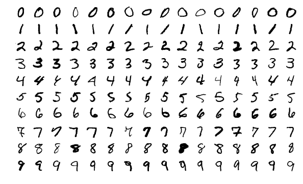
# Things seem to be as they should be. We have been able to accurately extract all the information necessary to read out all the remaining data stored in this file. Since these happen to be images, the accuracy of our read-out can be easily assessed by looking at the image content.
# In[6]:
n = 60000 # (anticipated) number of images.
d = 28*28 # number of entries (int values) per image.
times_todo = 5 # number of images to view.
bytes_left = d
data_x = np.zeros((d,), dtype=np.uint8) # initialize.
# Note that we are using the `uint8` (unsigned 1-byte int) data type, because we know that the values range between 0 and 255, based on the description by the authors of the data set, which says
#
# > "Pixels are organized row-wise. Pixel values are 0 to 255. 0 means background (white), 255 means foreground (black)."
# More concretely, we have that the remaining elements of the data set are of the form
# ```
# 0016 unsigned byte ?? pixel
# 0017 unsigned byte ?? pixel
# ........
# xxxx unsigned byte ?? pixel
# ```
# and so to read out one pixel value at a time (values between 0 and 255), we must read one byte at a time (rather than four bytes as we had just been doing). There should be $28 \times 28 = 784$ pixels per image.
# In[7]:
for t in range(times_todo):
idx = 0
while idx < bytes_left:
# Iterate one byte at a time.
b = f_bin.read(1)
data_x[idx] = int.from_bytes(b, byteorder="big", signed=False)
idx += 1
img_x = data_x.reshape( (28,28) ) # populate one row at a time.
# binary colour map highlights foreground (black) against background(white)
plt.imshow(img_x, cmap=plt.cm.binary)
#plt.savefig(("MNIST_train_"+str(t)+".png"))
plt.show()
f_bin.close()
if f_bin.closed:
print("Successfully closed.")
# __Exercises:__
#
# 0. When using the `from_bytes` method of `int`, change `signed` from `False` to `True`. Does the result of the binary to integer conversion change? If so, how? (provide examples) If possible, explain what causes this difference.
#
# 0. Similarly, change `byteorder` from `"big"` to `"little"`, and investigate if and how things change. Check `help(int.from_bytes)` for more information.
#
# 0. Note that there are countless colour maps (https://matplotlib.org/users/colormaps.html) available. Instead of `binary` as used, above try `gray`, `bone`, `pink`, and any others that catch your interest.
#
# 0. Uncomment the `savefig` line above, and save the first 10 training images to file. Then do the exact same procedure for *test* images, changing the file names appropriately.
#
# ___
#
# ## Examining the labels
#
# The images, or more generally, the *instances* to be used for the classification task appear as we expect. Let us now shift our focus over to the corresponding *labels* and confirm that the first `times_todo` instances indeed have the labels that we expect. These are stored in the `train-labels-idx1-ubyte` file.
# In[8]:
toread = "data/mnist/train-labels-idx1-ubyte"
f_bin = open(toread, mode="rb")
print(f_bin)
# Once again from the page of LeCun et al. linked above, we have for labels that the contents should be as follows.
#
# ```
# TRAINING SET LABEL FILE (train-labels-idx1-ubyte):
# [offset] [type] [value] [description]
# 0000 32 bit integer 0x00000801(2049) magic number (MSB first)
# 0004 32 bit integer 60000 number of items
# 0008 unsigned byte ?? label
# 0009 unsigned byte ?? label
# ........
# xxxx unsigned byte ?? label
# ```
#
# Let's inspect the first eight bytes.
# In[9]:
print("First four bytes:") # should be magic number, 2049.
b = f_bin.read(4)
print("bytes: ", b)
print(" int: ", int.from_bytes(b, byteorder="big"))
# In[10]:
print("Second four bytes:") # should be number of observations, 60000.
b = f_bin.read(4)
print("bytes: ", b)
print(" int: ", int.from_bytes(b, byteorder="big"))
# From here should be labels from 0 to 9. Let's confirm that the patterns above have correct labels corresponding to them in the place that we expect:
# In[11]:
times_todo = 5 # number of images to view.
for t in range(times_todo):
b = f_bin.read(1)
mylabel = int.from_bytes(b, byteorder="big", signed=False)
print("Label =", mylabel)
# __Exercises:__
#
# 0. Print out the label values for the first 10 images in both the training and testing data sets. Do these match the numbers that appear to be written in the images you saved to disk previously? (they should)
#
# 0. (Bonus) Instead of using `read`, we can use `seek` to jump to an arbitrary byte offset. In the example of instance labels above, `f_bin.seek(0)` would take us to the start of the file, and `f_bin.seek(8)` takes us to the point where the first label value is saved (since the first 8 bytes are clerical information). With this in mind, write a function that uses `seek` to display the label of the $k$th image, given integer $k$ only.
#
# 0. (Bonus) Similarly, write a function which uses `seek` to read and display the $k$th image itself, given just integer $k$.
# ___
#
# ## Prepare for training and evaluation
#
# Now, as an important practical concern, we will not want to have to open up the file and read pixel values byte-by-byte in the above fashion every time we want to train a classifier. A more reasonable approach is to read from the binary files just once, do any pre-processing that might be required, and store the data to be used for training and testing in a form that is fast to read.
#
# To do this, we use __PyTables__, a well-established Python package for managing hierarchical data sets and reading/writing large amounts of data [link]. The two-dimensional images will be stored simply as long vectors, contained within a 2D array whose rows correspond to distinct images. This array itself will be contained in a hierarchical data file that is quite convenient for fast reading.
# Let us start by reading the whole file.
# In[1]:
import tables
import numpy as np
import matplotlib.pyplot as plt
import os
# In[2]:
# Key information.
NUM_CLASSES = 10
NUM_LABELS = 1
NUM_PIXELS = 28*28
NUM_TRAIN = 60000
NUM_TEST = 10000
# In[3]:
# Open file connection, writing new file to disk.
myh5 = tables.open_file("data/mnist/data.h5",
mode="w",
title="MNIST handwritten digits with labels")
print(myh5) # currently empty.
# Within the `RootGroup`, we add two new groups for training and testing.
# In[4]:
myh5.create_group(myh5.root, "train", "Training data")
myh5.create_group(myh5.root, "test", "Testing data")
print(myh5)
# Within `train` and `test`, prepare *enumerative array* (`EArray` class) objects which will be used for storing data. Enumerative arrays are different from typical `Array` objects in that new data can be added freely at a later date.
# In[5]:
# Training data arrays.
a = tables.UInt8Atom()
myh5.create_earray(myh5.root.train,
name="labels",
atom=a,
shape=(0,NUM_LABELS),
title="Label values")
a = tables.Float32Atom()
myh5.create_earray(myh5.root.train,
name="inputs",
atom=a,
shape=(0,NUM_PIXELS),
title="Input images")
# Testing data arrays.
a = tables.UInt8Atom()
myh5.create_earray(myh5.root.test,
name="labels",
atom=a,
shape=(0,NUM_LABELS),
title="Label values")
a = tables.Float32Atom()
myh5.create_earray(myh5.root.test,
name="inputs",
atom=a,
shape=(0,NUM_PIXELS),
title="Input images")
print(myh5)
# The arrays are ready to be populated. Note that the first dimension is the "enlargeable dimension". It starts with no entries and is thus zero, but grows as we append data. First, we need to read the data, then we will do a bit of pre-processing.
# In[6]:
toread = "data/mnist/train-images-idx3-ubyte"
bytes_left = NUM_TRAIN*NUM_PIXELS
data_X = np.empty((NUM_TRAIN*NUM_PIXELS,), dtype=np.uint8)
with open(toread, mode="rb") as f_bin:
f_bin.seek(16) # go to start of images.
idx = 0
print("Reading binary file...", end=" ")
while bytes_left > 0:
b = f_bin.read(1)
data_X[idx] = int.from_bytes(b, byteorder="big", signed=False)
bytes_left -= 1
idx += 1
print("Done reading...", end=" ")
print("OK, file closed.")
data_X = data_X.reshape((NUM_TRAIN,NUM_PIXELS))
# Using the unsigned integer `uint8` data type, we have assembled all pixel values for all instances in one long vector. Let's examine basic statistics:
# In[7]:
print("Statistics before pre-processing:")
print("Min:", np.min(data_X))
print("Mean:", np.mean(data_X))
print("Median:", np.median(data_X))
print("Max:", np.max(data_X))
print("StdDev:", np.std(data_X))
#print(np.bincount(data_X))
# Certain models run into numerical difficulties if the input features are too large. Here they range over $\{0,1,\ldots,255\}$, which can lead to huge values when, for example, passed through exponential functions (e.g., logistic regression). To get around this, it is useful to map the values to the unit interval $[0,1]$. The basic formula is simple: (VALUE - MIN) / (MAX - MIN). We will use more memory to store floating point numbers, but computation in learning tasks is often made considerably easier.
# In[8]:
data_X = np.float32(data_X)
data_X = (data_X - np.min(data_X)) / (np.max(data_X) - np.min(data_X))
print("Statistics after pre-processing:")
print("Min:", np.min(data_X))
print("Mean:", np.mean(data_X))
print("Median:", np.median(data_X))
print("Max:", np.max(data_X))
print("StdDev:", np.std(data_X))
# Let us now also read the training labels from disk; note that the labels take the form $0,1,\ldots,9$, which is convenient for our later computations, and no pre-processing is required.
# In[9]:
toread = "data/mnist/train-labels-idx1-ubyte"
bytes_left = NUM_TRAIN
data_y = np.zeros((NUM_TRAIN,1), dtype=np.uint8)
with open(toread, mode="rb") as f_bin:
f_bin.seek(8) # go to start of the labels.
idx = 0
print("Reading binary file...", end=" ")
while bytes_left > 0:
b = f_bin.read(1)
data_y[idx,0] = int.from_bytes(b, byteorder="big", signed=False)
bytes_left -= 1
idx += 1
print("Done reading...", end=" ")
print("OK, file closed.")
# In[10]:
print("Min:", np.min(data_y))
print("Mean:", np.mean(data_y))
print("Median:", np.median(data_y))
print("Max:", np.max(data_y))
print("StdDev:", np.std(data_y))
print("Bin counts:")
print(np.bincount(data_y[:,0]))
plt.hist(np.hstack(data_y), bins='auto')
plt.show()
# Now let us append the data to the hierarchical data file we initialized.
# In[11]:
for i in range(NUM_TRAIN):
myh5.root.train.inputs.append([data_X[i,:]])
myh5.root.train.labels.append([data_y[i,:]])
# Having run the above code, we can clearly see that the desired number of observations have been added to the arrays under the `train` group.
# In[12]:
print(myh5)
# Now we just repeat this for the testing data.
# In[13]:
toread = "data/mnist/t10k-images-idx3-ubyte"
bytes_left = NUM_TEST*NUM_PIXELS
data_X = np.empty((NUM_TEST*NUM_PIXELS,), dtype=np.uint8)
with open(toread, mode="rb") as f_bin:
f_bin.seek(16) # go to start of images.
idx = 0
print("Reading binary file...", end=" ")
while bytes_left > 0:
b = f_bin.read(1)
data_X[idx] = int.from_bytes(b, byteorder="big", signed=False)
bytes_left -= 1
idx += 1
print("Done reading...", end=" ")
print("OK, file closed.")
data_X = data_X.reshape((NUM_TEST,NUM_PIXELS))
data_X = np.float32(data_X)
data_X = (data_X - np.min(data_X)) / (np.max(data_X) - np.min(data_X))
toread = "data/mnist/t10k-labels-idx1-ubyte"
bytes_left = NUM_TEST
data_y = np.zeros((NUM_TEST,1), dtype=np.uint8)
with open(toread, mode="rb") as f_bin:
f_bin.seek(8) # go to start of the labels.
idx = 0
print("Reading binary file...", end=" ")
while bytes_left > 0:
b = f_bin.read(1)
data_y[idx,0] = int.from_bytes(b, byteorder="big", signed=False)
bytes_left -= 1
idx += 1
print("Done reading...", end=" ")
print("OK, file closed.")
# In[14]:
for i in range(NUM_TEST):
myh5.root.test.inputs.append([data_X[i,:]])
myh5.root.test.labels.append([data_y[i,:]])
# In[15]:
print(myh5)
# Finally, be sure to close the file connection.
# In[16]:
myh5.close()
# __Exercises:__
#
# 0. Re-open the connection with the file we just made in *read* mode (`mode="r"`). Read out the first few image vectors and their labels, and ensure that they have been saved as we expect.
# ___
# A typical source for this data set is the website of Y. LeCun ( http://yann.lecun.com/exdb/mnist/ ). They provide the following description,
#
# > *"The MNIST database of handwritten digits, available from this page, has a training set of 60,000 examples, and a test set of 10,000 examples. It is a subset of a larger set available from NIST. The digits have been size-normalized and centered in a fixed-size image"*
# and the following files containing the data of interest.
#
# > train-images-idx3-ubyte.gz: training set images (9912422 bytes)
# > train-labels-idx1-ubyte.gz: training set labels (28881 bytes)
# > t10k-images-idx3-ubyte.gz: test set images (1648877 bytes)
# > t10k-labels-idx1-ubyte.gz: test set labels (4542 bytes)
# The files are stored in a binary format called __IDX__, typically used for storing vector data. First we decompress the files via
#
# ```
# $ cd data/mnist
# $ gunzip train-images-idx3-ubyte.gz
# $ gunzip train-labels-idx1-ubyte.gz
# $ gunzip t10k-images-idx3-ubyte.gz
# $ gunzip t10k-labels-idx1-ubyte.gz
# ```
# which leaves us with the desired binary files.
#
# ___
#
# ## Examining the input patterns
#
# Let us begin by opening a file connection with the training examples.
#
# In[1]:
import numpy as np
import matplotlib.pyplot as plt
toread = "data/mnist/train-images-idx3-ubyte"
f_bin = open(toread, mode="rb")
print(f_bin)
# Now, in order to ensure that we are reading the data correctly, the only way to confirm this is by inspecting and checking with what the authors of the data file tell us *should* be there. From the page of LeCun et al. linked above, we have the following:
# ```
# TRAINING SET IMAGE FILE (train-images-idx3-ubyte):
# [offset] [type] [value] [description]
# 0000 32 bit integer 0x00000803(2051) magic number
# 0004 32 bit integer 60000 number of images
# 0008 32 bit integer 28 number of rows
# 0012 32 bit integer 28 number of columns
# 0016 unsigned byte ?? pixel
# 0017 unsigned byte ?? pixel
# ........
# xxxx unsigned byte ?? pixel
# ```
# The "offset" here refers to the number of bytes read from the start of the file. An offset of zero refers to the first byte, and an offset of 0004 refers to the fifth byte, 0008 the ninth byte, and so forth. Let's check that we are able to successfully read what we expect.
# In[2]:
print("First four bytes:") # should be magic number, 2051.
b = f_bin.read(4)
print("bytes: ", b)
print(" int: ", int.from_bytes(b, byteorder="big", signed=False))
# Note that the byte data `b'\x00\x00\x08\x03'` shown here by Python is a hexadecimal representation of the first four bytes. This corresponds directly to the "value" in the first row of the table above, ``0x00000803``. The ``\x`` breaks simply show where one byte starts and another ends, recalling that using two hexadecimal digits we can represent the integers from $0, 1, 2, \ldots$ through to $(15 \times 16^{1} + 15 \times 16^{0}) = 255$, just as we can with 8 binary digits, or 8 *bits*. Anyways, converting this to decimal, $3 \times 16^{0} + 8 \times 16^{2} = 2051$, precisely what we expect.
# Using the *read* method, let us read four bytes at a time to ensure the remaining data is read correctly.
# In[3]:
print("Second four bytes:") # should be number of imgs = 60000
b = f_bin.read(4)
print("bytes: ", b)
print(" int: ", int.from_bytes(b, byteorder="big", signed=False))
# In[4]:
print("Third four bytes:") # should be number of rows = 28
b = f_bin.read(4)
print("bytes: ", b)
print(" int: ", int.from_bytes(b, byteorder="big", signed=False))
# In[5]:
print("Fourth four bytes:") # should be number of cols = 28
b = f_bin.read(4)
print("bytes: ", b)
print(" int: ", int.from_bytes(b, byteorder="big", signed=False))
# Things seem to be as they should be. We have been able to accurately extract all the information necessary to read out all the remaining data stored in this file. Since these happen to be images, the accuracy of our read-out can be easily assessed by looking at the image content.
# In[6]:
n = 60000 # (anticipated) number of images.
d = 28*28 # number of entries (int values) per image.
times_todo = 5 # number of images to view.
bytes_left = d
data_x = np.zeros((d,), dtype=np.uint8) # initialize.
# Note that we are using the `uint8` (unsigned 1-byte int) data type, because we know that the values range between 0 and 255, based on the description by the authors of the data set, which says
#
# > "Pixels are organized row-wise. Pixel values are 0 to 255. 0 means background (white), 255 means foreground (black)."
# More concretely, we have that the remaining elements of the data set are of the form
# ```
# 0016 unsigned byte ?? pixel
# 0017 unsigned byte ?? pixel
# ........
# xxxx unsigned byte ?? pixel
# ```
# and so to read out one pixel value at a time (values between 0 and 255), we must read one byte at a time (rather than four bytes as we had just been doing). There should be $28 \times 28 = 784$ pixels per image.
# In[7]:
for t in range(times_todo):
idx = 0
while idx < bytes_left:
# Iterate one byte at a time.
b = f_bin.read(1)
data_x[idx] = int.from_bytes(b, byteorder="big", signed=False)
idx += 1
img_x = data_x.reshape( (28,28) ) # populate one row at a time.
# binary colour map highlights foreground (black) against background(white)
plt.imshow(img_x, cmap=plt.cm.binary)
#plt.savefig(("MNIST_train_"+str(t)+".png"))
plt.show()
f_bin.close()
if f_bin.closed:
print("Successfully closed.")
# __Exercises:__
#
# 0. When using the `from_bytes` method of `int`, change `signed` from `False` to `True`. Does the result of the binary to integer conversion change? If so, how? (provide examples) If possible, explain what causes this difference.
#
# 0. Similarly, change `byteorder` from `"big"` to `"little"`, and investigate if and how things change. Check `help(int.from_bytes)` for more information.
#
# 0. Note that there are countless colour maps (https://matplotlib.org/users/colormaps.html) available. Instead of `binary` as used, above try `gray`, `bone`, `pink`, and any others that catch your interest.
#
# 0. Uncomment the `savefig` line above, and save the first 10 training images to file. Then do the exact same procedure for *test* images, changing the file names appropriately.
#
# ___
#
# ## Examining the labels
#
# The images, or more generally, the *instances* to be used for the classification task appear as we expect. Let us now shift our focus over to the corresponding *labels* and confirm that the first `times_todo` instances indeed have the labels that we expect. These are stored in the `train-labels-idx1-ubyte` file.
# In[8]:
toread = "data/mnist/train-labels-idx1-ubyte"
f_bin = open(toread, mode="rb")
print(f_bin)
# Once again from the page of LeCun et al. linked above, we have for labels that the contents should be as follows.
#
# ```
# TRAINING SET LABEL FILE (train-labels-idx1-ubyte):
# [offset] [type] [value] [description]
# 0000 32 bit integer 0x00000801(2049) magic number (MSB first)
# 0004 32 bit integer 60000 number of items
# 0008 unsigned byte ?? label
# 0009 unsigned byte ?? label
# ........
# xxxx unsigned byte ?? label
# ```
#
# Let's inspect the first eight bytes.
# In[9]:
print("First four bytes:") # should be magic number, 2049.
b = f_bin.read(4)
print("bytes: ", b)
print(" int: ", int.from_bytes(b, byteorder="big"))
# In[10]:
print("Second four bytes:") # should be number of observations, 60000.
b = f_bin.read(4)
print("bytes: ", b)
print(" int: ", int.from_bytes(b, byteorder="big"))
# From here should be labels from 0 to 9. Let's confirm that the patterns above have correct labels corresponding to them in the place that we expect:
# In[11]:
times_todo = 5 # number of images to view.
for t in range(times_todo):
b = f_bin.read(1)
mylabel = int.from_bytes(b, byteorder="big", signed=False)
print("Label =", mylabel)
# __Exercises:__
#
# 0. Print out the label values for the first 10 images in both the training and testing data sets. Do these match the numbers that appear to be written in the images you saved to disk previously? (they should)
#
# 0. (Bonus) Instead of using `read`, we can use `seek` to jump to an arbitrary byte offset. In the example of instance labels above, `f_bin.seek(0)` would take us to the start of the file, and `f_bin.seek(8)` takes us to the point where the first label value is saved (since the first 8 bytes are clerical information). With this in mind, write a function that uses `seek` to display the label of the $k$th image, given integer $k$ only.
#
# 0. (Bonus) Similarly, write a function which uses `seek` to read and display the $k$th image itself, given just integer $k$.
# ___
#
# ## Prepare for training and evaluation
#
# Now, as an important practical concern, we will not want to have to open up the file and read pixel values byte-by-byte in the above fashion every time we want to train a classifier. A more reasonable approach is to read from the binary files just once, do any pre-processing that might be required, and store the data to be used for training and testing in a form that is fast to read.
#
# To do this, we use __PyTables__, a well-established Python package for managing hierarchical data sets and reading/writing large amounts of data [link]. The two-dimensional images will be stored simply as long vectors, contained within a 2D array whose rows correspond to distinct images. This array itself will be contained in a hierarchical data file that is quite convenient for fast reading.
# Let us start by reading the whole file.
# In[1]:
import tables
import numpy as np
import matplotlib.pyplot as plt
import os
# In[2]:
# Key information.
NUM_CLASSES = 10
NUM_LABELS = 1
NUM_PIXELS = 28*28
NUM_TRAIN = 60000
NUM_TEST = 10000
# In[3]:
# Open file connection, writing new file to disk.
myh5 = tables.open_file("data/mnist/data.h5",
mode="w",
title="MNIST handwritten digits with labels")
print(myh5) # currently empty.
# Within the `RootGroup`, we add two new groups for training and testing.
# In[4]:
myh5.create_group(myh5.root, "train", "Training data")
myh5.create_group(myh5.root, "test", "Testing data")
print(myh5)
# Within `train` and `test`, prepare *enumerative array* (`EArray` class) objects which will be used for storing data. Enumerative arrays are different from typical `Array` objects in that new data can be added freely at a later date.
# In[5]:
# Training data arrays.
a = tables.UInt8Atom()
myh5.create_earray(myh5.root.train,
name="labels",
atom=a,
shape=(0,NUM_LABELS),
title="Label values")
a = tables.Float32Atom()
myh5.create_earray(myh5.root.train,
name="inputs",
atom=a,
shape=(0,NUM_PIXELS),
title="Input images")
# Testing data arrays.
a = tables.UInt8Atom()
myh5.create_earray(myh5.root.test,
name="labels",
atom=a,
shape=(0,NUM_LABELS),
title="Label values")
a = tables.Float32Atom()
myh5.create_earray(myh5.root.test,
name="inputs",
atom=a,
shape=(0,NUM_PIXELS),
title="Input images")
print(myh5)
# The arrays are ready to be populated. Note that the first dimension is the "enlargeable dimension". It starts with no entries and is thus zero, but grows as we append data. First, we need to read the data, then we will do a bit of pre-processing.
# In[6]:
toread = "data/mnist/train-images-idx3-ubyte"
bytes_left = NUM_TRAIN*NUM_PIXELS
data_X = np.empty((NUM_TRAIN*NUM_PIXELS,), dtype=np.uint8)
with open(toread, mode="rb") as f_bin:
f_bin.seek(16) # go to start of images.
idx = 0
print("Reading binary file...", end=" ")
while bytes_left > 0:
b = f_bin.read(1)
data_X[idx] = int.from_bytes(b, byteorder="big", signed=False)
bytes_left -= 1
idx += 1
print("Done reading...", end=" ")
print("OK, file closed.")
data_X = data_X.reshape((NUM_TRAIN,NUM_PIXELS))
# Using the unsigned integer `uint8` data type, we have assembled all pixel values for all instances in one long vector. Let's examine basic statistics:
# In[7]:
print("Statistics before pre-processing:")
print("Min:", np.min(data_X))
print("Mean:", np.mean(data_X))
print("Median:", np.median(data_X))
print("Max:", np.max(data_X))
print("StdDev:", np.std(data_X))
#print(np.bincount(data_X))
# Certain models run into numerical difficulties if the input features are too large. Here they range over $\{0,1,\ldots,255\}$, which can lead to huge values when, for example, passed through exponential functions (e.g., logistic regression). To get around this, it is useful to map the values to the unit interval $[0,1]$. The basic formula is simple: (VALUE - MIN) / (MAX - MIN). We will use more memory to store floating point numbers, but computation in learning tasks is often made considerably easier.
# In[8]:
data_X = np.float32(data_X)
data_X = (data_X - np.min(data_X)) / (np.max(data_X) - np.min(data_X))
print("Statistics after pre-processing:")
print("Min:", np.min(data_X))
print("Mean:", np.mean(data_X))
print("Median:", np.median(data_X))
print("Max:", np.max(data_X))
print("StdDev:", np.std(data_X))
# Let us now also read the training labels from disk; note that the labels take the form $0,1,\ldots,9$, which is convenient for our later computations, and no pre-processing is required.
# In[9]:
toread = "data/mnist/train-labels-idx1-ubyte"
bytes_left = NUM_TRAIN
data_y = np.zeros((NUM_TRAIN,1), dtype=np.uint8)
with open(toread, mode="rb") as f_bin:
f_bin.seek(8) # go to start of the labels.
idx = 0
print("Reading binary file...", end=" ")
while bytes_left > 0:
b = f_bin.read(1)
data_y[idx,0] = int.from_bytes(b, byteorder="big", signed=False)
bytes_left -= 1
idx += 1
print("Done reading...", end=" ")
print("OK, file closed.")
# In[10]:
print("Min:", np.min(data_y))
print("Mean:", np.mean(data_y))
print("Median:", np.median(data_y))
print("Max:", np.max(data_y))
print("StdDev:", np.std(data_y))
print("Bin counts:")
print(np.bincount(data_y[:,0]))
plt.hist(np.hstack(data_y), bins='auto')
plt.show()
# Now let us append the data to the hierarchical data file we initialized.
# In[11]:
for i in range(NUM_TRAIN):
myh5.root.train.inputs.append([data_X[i,:]])
myh5.root.train.labels.append([data_y[i,:]])
# Having run the above code, we can clearly see that the desired number of observations have been added to the arrays under the `train` group.
# In[12]:
print(myh5)
# Now we just repeat this for the testing data.
# In[13]:
toread = "data/mnist/t10k-images-idx3-ubyte"
bytes_left = NUM_TEST*NUM_PIXELS
data_X = np.empty((NUM_TEST*NUM_PIXELS,), dtype=np.uint8)
with open(toread, mode="rb") as f_bin:
f_bin.seek(16) # go to start of images.
idx = 0
print("Reading binary file...", end=" ")
while bytes_left > 0:
b = f_bin.read(1)
data_X[idx] = int.from_bytes(b, byteorder="big", signed=False)
bytes_left -= 1
idx += 1
print("Done reading...", end=" ")
print("OK, file closed.")
data_X = data_X.reshape((NUM_TEST,NUM_PIXELS))
data_X = np.float32(data_X)
data_X = (data_X - np.min(data_X)) / (np.max(data_X) - np.min(data_X))
toread = "data/mnist/t10k-labels-idx1-ubyte"
bytes_left = NUM_TEST
data_y = np.zeros((NUM_TEST,1), dtype=np.uint8)
with open(toread, mode="rb") as f_bin:
f_bin.seek(8) # go to start of the labels.
idx = 0
print("Reading binary file...", end=" ")
while bytes_left > 0:
b = f_bin.read(1)
data_y[idx,0] = int.from_bytes(b, byteorder="big", signed=False)
bytes_left -= 1
idx += 1
print("Done reading...", end=" ")
print("OK, file closed.")
# In[14]:
for i in range(NUM_TEST):
myh5.root.test.inputs.append([data_X[i,:]])
myh5.root.test.labels.append([data_y[i,:]])
# In[15]:
print(myh5)
# Finally, be sure to close the file connection.
# In[16]:
myh5.close()
# __Exercises:__
#
# 0. Re-open the connection with the file we just made in *read* mode (`mode="r"`). Read out the first few image vectors and their labels, and ensure that they have been saved as we expect.
# ___