#!/usr/bin/env python
# coding: utf-8
# # CIFAR-10 tiny images
#
# The *CIFAR-10* data set is a collection of tiny digital images, with simple text labels assigned to each image, reflecting the content of the image.
# __Contents:__
# - Overview of the data set
# - Examining the (image, label) pairs
# - Prepare for training and evaluation
# ___
#
# ## Overview of the data set
#
# At present (July 2018), the CIFAR-10 data set is hosted by the University of Toronto, and is easily accessed via the home page of Alex Krizhevsky:
#
# ```
# http://www.cs.toronto.edu/~kriz/cifar.html
# ```
#
# This dataset is a subset of the *Tiny Images* dataset, a large data set of nearly 80 million images with thousands of distinct labels [link]. For reference, __CIFAR__ is an acronym, and stands for the (C)anadian (I)nstitute (for (A)dvanced (R)esearch.
#
# The CIFAR-10 dataset is typically used for training image classification systems, and includes just ten distinct labels: *airplane*, *automobile*, *bird*, *cat*, *deer*, *dog*, *frog*, *horse*, *ship*, and *truck*. See an example below:
# 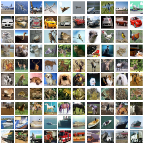 # Basic facts:
#
# - 60,000 images
# - 32x32 colour images
# - 10 classes
# - Balanced classes (6,000 images per class)
#
# Having acquired the data, let's get started. Within the directory `cifar-10-batches-bin`, we have the following content:
#
# ```
# $ ls cifar-10-batches-bin
# batches.meta.txt data_batch_2.bin data_batch_4.bin readme.html
# data_batch_1.bin data_batch_3.bin data_batch_5.bin test_batch.bin
# ```
#
# The `batches.meta.txt` file just contains label names, one per line. What remains are six batches in binary format: five training batches (`data_batch_*.bin`) and one test batch (`test_batch.bin`). Each batch has 10,000 images. Regarding the balance of classes:
#
# > The test batch contains exactly 1000 randomly-selected images from each class. The training batches contain the remaining images in random order, but some training batches may contain more images from one class than another. Between them, the training batches contain exactly 5000 images from each class.
#
# Time to dig in to the binary files.
#
# ## Examining the (image, label) pairs
#
# Let us begin by opening a file connection with the training examples.
#
# In[1]:
import numpy as np
import matplotlib.pyplot as plt
toread = "data/cifar10/cifar-10-batches-bin/data_batch_1.bin"
f_bin = open(toread, mode="rb")
print(f_bin)
# Next we make sure that we know how to read the data correctly. The only way to do this is to confirm by inspection, verifying that the content we read is the content the authors tell us we should be reading. From the documentation, the file format is extremely simple:
#
# - The basic format is `<1 x label><3072 x pixel>`, namely one byte containing the label, and 3072 bytes containing pixel information. Thus the first 3073 bytes contain all the information required for the first (image,label) pair. This "row" of data occurs 10,000 times per batch.
# - Labels are integers between 0 and 9.
# - Images are 32 x 32 = 1024 pixels, one byte per pixel. These pixel values are stored one colour channel at a time: red, green, blue.
# - Values are stored in *row-major* order, so we populate by rows, rather than by columns.
#
# This is enough information to get started.
# In[2]:
print("First byte:") # should be a label.
b = f_bin.read(1)
print("bytes: ", b)
print("int: ", int.from_bytes(b, byteorder="big", signed=False))
# Note that the byte data `b'\x06'` shown here by Python is a hexadecimal representation of the first byte. The ``\x`` breaks simply show where one byte starts and another ends, recalling that using two hexadecimal digits we can represent the integers from $0, 1, 2, \ldots$ through to $(15 \times 16^{1} + 15 \times 16^{0}) = 255$, just as we can with 8 binary digits, or 1 *byte*.
#
# Let's look at the content of the next five pixel values, assuming they are unsigned integers.
# In[3]:
for i in range(5):
b = f_bin.read(1)
print("bytes: ", b)
print("int: ", int.from_bytes(b, byteorder="big", signed=False))
# First, note that while `b';'` may appear a bit strange, Python uses ASCII characters whenever possible instead of a typical hexadecimal representation. What is important is the resulting integer values. At this point, we can see that the values are similar, but we certainly do not know that they are correct yet. Let's `seek()` back to the first pixel value, and read out the whole image into a numpy array.
# In[4]:
f_bin.seek(1)
my_array = np.zeros((32,32,3), dtype=np.uint8)
for c in range(3): # colour channel
for i in range(32): # rows
for j in range(32): # columns
b = f_bin.read(1)
my_array[i,j,c] = int.from_bytes(b, byteorder="big", signed=False)
# In[5]:
plt.imshow(my_array)
# This looks like an image of a frog. The label is 6, namely the seventh label, and from the file `batches.meta.txt` we have
#
# ```
# $ cat batches.meta.txt
# airplane
# automobile
# bird
# cat
# deer
# dog
# frog
# horse
# ship
# truck
# ```
#
# which lets us confirm that the label is as we expect. Let's do one more (image,label) pair.
# In[6]:
b = f_bin.read(1)
print("bytes: ", b)
print("int: ", int.from_bytes(b, byteorder="big", signed=False))
my_array = np.zeros((32,32,3), dtype=np.uint8)
for c in range(3): # colour channel
for i in range(32): # rows
for j in range(32): # columns
b = f_bin.read(1)
my_array[i,j,c] = int.from_bytes(b, byteorder="big", signed=False)
# In[7]:
plt.imshow(my_array)
# We have an image of a truck, with label value 9, the tenth label. This is precisely as we would expect. Let's close the file for now, and proceed with processing the entire data set.
#
# ## Prepare for training and evaluation
#
# In the previous section, we used 3D arrays for visualizing the image contents. For learning, each image will just be a long vector, contained within a 2D array whose rows correspond to distinct images. This array itself will be contained in a hierarchical data file that is quite convenient for fast reading. To do this, we use __PyTables__, a well-established Python package for managing hierarchical data sets and reading/writing large amounts of data [link].
#
# We begin by generating a new file.
# In[1]:
import tables
import numpy as np
import matplotlib.pyplot as plt
import os
# In[2]:
# Key information.
NUM_CLASSES = 10
NUM_LABELS = 1
NUM_PIXELS = 32*32
NUM_CHANNELS = 3
NUM_BATCHIM = 10000 # number of images per batch.
# A dictionary mapping label values (ints) to strings.
toread = "data/cifar10/cifar-10-batches-bin/batches.meta.txt"
LABEL_DICT = {}
with open(toread, mode="r", encoding="ascii") as f:
for cnt, line in enumerate(f):
LABEL_DICT[cnt] = line.split("\n")[0] # to remove the line-breaks.
LABEL_DICT.pop(10) # to remove the empty line.
# In[3]:
# Open file connection, writing new file to disk.
myh5 = tables.open_file("data/cifar10/data.h5",
mode="w",
title="CIFAR-10 data")
print(myh5) # currently empty.
# Within the `RootGroup`, let us add two new groups for training and testing.
# In[4]:
myh5.create_group(myh5.root, "train", "Training data")
myh5.create_group(myh5.root, "test", "Testing data")
print(myh5)
# Within `train` and `test`, prepare *enumerative array* (`EArray` class) objects which will be used for storing data. Enumerative arrays are different from typical `Array` objects in that new data can be added freely at a later date.
# In[5]:
# Training data arrays.
a = tables.UInt8Atom()
myh5.create_earray(myh5.root.train,
name="labels",
atom=a,
shape=(0,NUM_LABELS),
title="Label values")
a = tables.Float32Atom()
myh5.create_earray(myh5.root.train,
name="inputs",
atom=a,
shape=(0,NUM_CHANNELS*NUM_PIXELS),
title="Input images")
# Testing data arrays.
a = tables.UInt8Atom()
myh5.create_earray(myh5.root.test,
name="labels",
atom=a,
shape=(0,NUM_LABELS),
title="Label values")
a = tables.Float32Atom()
myh5.create_earray(myh5.root.test,
name="inputs",
atom=a,
shape=(0,NUM_CHANNELS*NUM_PIXELS),
title="Input images")
print(myh5)
# The arrays are ready to be populated. Note that the first dimension is the "enlargeable dimension". It starts with no entries and is thus zero, but grows as we append data.
#
# We shall carry out just one simple bit of pre-processing: normalization of pixel values to the unit interval $[0,1]$. This is accomplished by dividing existing pixels by 255. We handle all training batches at once, as below.
# In[7]:
def process_inputs(x):
'''
Normalization of the inputs.
'''
return np.float32(x/255.0)
# In[10]:
todo_batches = [1, 2]
# Storage preparation.
datum_input = np.zeros((NUM_CHANNELS*NUM_PIXELS,), dtype=np.float32)
datum_label = np.zeros((1,), dtype=np.uint8)
# Loop over the batch itinerary.
for bt in todo_batches:
fname = "data_batch_" + str(bt) + ".bin"
toread = os.path.join("data", "cifar10", "cifar-10-batches-bin", fname)
f_bin = open(toread, mode="rb")
print("--", "BATCH", bt, "--")
for i in range(NUM_BATCHIM):
if i % 1000 == 0:
print("Working... image", i)
b = f_bin.read(1)
datum_label[0] = int.from_bytes(b, byteorder="big", signed=False)
for j in range(NUM_CHANNELS*NUM_PIXELS):
# Populate a long vector.
b = f_bin.read(1)
datum_input[j] = int.from_bytes(b, byteorder="big", signed=False)
# Append.
myh5.root.train.inputs.append([process_inputs(datum_input)]) # inputs
myh5.root.train.labels.append([datum_label]) # labels
f_bin.close()
# Having run the above code, we can clearly see that the desired number of observations have been added to the arrays under the `train` group.
# In[11]:
print(myh5)
# Let's do the same thing for the `test` group below.
# In[12]:
# Storage preparation.
datum_input = np.zeros((NUM_CHANNELS*NUM_PIXELS,), dtype=np.float32)
datum_label = np.zeros((1,), dtype=np.uint8)
# Loop over the batch itinerary.
fname = "test_batch.bin"
toread = os.path.join("data", "cifar10", "cifar-10-batches-bin", fname)
f_bin = open(toread, mode="rb")
print("--", "TEST BATCH", "--")
for i in range(NUM_BATCHIM):
if i % 1000 == 0:
print("Working... image", i)
b = f_bin.read(1)
datum_label[0] = int.from_bytes(b, byteorder="big", signed=False)
for j in range(NUM_CHANNELS*NUM_PIXELS):
# Populate a long vector.
b = f_bin.read(1)
datum_input[j] = int.from_bytes(b, byteorder="big", signed=False)
# Append.
myh5.root.test.inputs.append([process_inputs(datum_input)]) # inputs
myh5.root.test.labels.append([datum_label]) # labels
f_bin.close()
# Let's do one final check of the content, and close the final connection.
# In[13]:
print(myh5)
myh5.close()
# Finally, let us ensure that our new file houses data in the form that we expect.
# In[21]:
# Read an arbitrary image.
f = tables.open_file("data/cifar10/data.h5", mode="r")
todo_vals = [1509, 1959, 1988, 9018]
for i in range(len(todo_vals)):
todo = todo_vals[i]
myinput = f.root.train.inputs.read(start=todo, stop=(todo+1), step=1)
mylabel = f.root.train.labels.read(start=todo, stop=(todo+1), step=1)
myim = myinput.flatten().reshape((3,32,32))
myim = np.swapaxes(myim, 0, 1) # note the axis swapping.
myim = np.swapaxes(myim, 1, 2) # note the axis swapping.
plt.imshow(myim)
plt.show()
print("LABEL:", mylabel[0][0], "=", LABEL_DICT[mylabel[0][0]])
f.close()
# ___
# Basic facts:
#
# - 60,000 images
# - 32x32 colour images
# - 10 classes
# - Balanced classes (6,000 images per class)
#
# Having acquired the data, let's get started. Within the directory `cifar-10-batches-bin`, we have the following content:
#
# ```
# $ ls cifar-10-batches-bin
# batches.meta.txt data_batch_2.bin data_batch_4.bin readme.html
# data_batch_1.bin data_batch_3.bin data_batch_5.bin test_batch.bin
# ```
#
# The `batches.meta.txt` file just contains label names, one per line. What remains are six batches in binary format: five training batches (`data_batch_*.bin`) and one test batch (`test_batch.bin`). Each batch has 10,000 images. Regarding the balance of classes:
#
# > The test batch contains exactly 1000 randomly-selected images from each class. The training batches contain the remaining images in random order, but some training batches may contain more images from one class than another. Between them, the training batches contain exactly 5000 images from each class.
#
# Time to dig in to the binary files.
#
# ## Examining the (image, label) pairs
#
# Let us begin by opening a file connection with the training examples.
#
# In[1]:
import numpy as np
import matplotlib.pyplot as plt
toread = "data/cifar10/cifar-10-batches-bin/data_batch_1.bin"
f_bin = open(toread, mode="rb")
print(f_bin)
# Next we make sure that we know how to read the data correctly. The only way to do this is to confirm by inspection, verifying that the content we read is the content the authors tell us we should be reading. From the documentation, the file format is extremely simple:
#
# - The basic format is `<1 x label><3072 x pixel>`, namely one byte containing the label, and 3072 bytes containing pixel information. Thus the first 3073 bytes contain all the information required for the first (image,label) pair. This "row" of data occurs 10,000 times per batch.
# - Labels are integers between 0 and 9.
# - Images are 32 x 32 = 1024 pixels, one byte per pixel. These pixel values are stored one colour channel at a time: red, green, blue.
# - Values are stored in *row-major* order, so we populate by rows, rather than by columns.
#
# This is enough information to get started.
# In[2]:
print("First byte:") # should be a label.
b = f_bin.read(1)
print("bytes: ", b)
print("int: ", int.from_bytes(b, byteorder="big", signed=False))
# Note that the byte data `b'\x06'` shown here by Python is a hexadecimal representation of the first byte. The ``\x`` breaks simply show where one byte starts and another ends, recalling that using two hexadecimal digits we can represent the integers from $0, 1, 2, \ldots$ through to $(15 \times 16^{1} + 15 \times 16^{0}) = 255$, just as we can with 8 binary digits, or 1 *byte*.
#
# Let's look at the content of the next five pixel values, assuming they are unsigned integers.
# In[3]:
for i in range(5):
b = f_bin.read(1)
print("bytes: ", b)
print("int: ", int.from_bytes(b, byteorder="big", signed=False))
# First, note that while `b';'` may appear a bit strange, Python uses ASCII characters whenever possible instead of a typical hexadecimal representation. What is important is the resulting integer values. At this point, we can see that the values are similar, but we certainly do not know that they are correct yet. Let's `seek()` back to the first pixel value, and read out the whole image into a numpy array.
# In[4]:
f_bin.seek(1)
my_array = np.zeros((32,32,3), dtype=np.uint8)
for c in range(3): # colour channel
for i in range(32): # rows
for j in range(32): # columns
b = f_bin.read(1)
my_array[i,j,c] = int.from_bytes(b, byteorder="big", signed=False)
# In[5]:
plt.imshow(my_array)
# This looks like an image of a frog. The label is 6, namely the seventh label, and from the file `batches.meta.txt` we have
#
# ```
# $ cat batches.meta.txt
# airplane
# automobile
# bird
# cat
# deer
# dog
# frog
# horse
# ship
# truck
# ```
#
# which lets us confirm that the label is as we expect. Let's do one more (image,label) pair.
# In[6]:
b = f_bin.read(1)
print("bytes: ", b)
print("int: ", int.from_bytes(b, byteorder="big", signed=False))
my_array = np.zeros((32,32,3), dtype=np.uint8)
for c in range(3): # colour channel
for i in range(32): # rows
for j in range(32): # columns
b = f_bin.read(1)
my_array[i,j,c] = int.from_bytes(b, byteorder="big", signed=False)
# In[7]:
plt.imshow(my_array)
# We have an image of a truck, with label value 9, the tenth label. This is precisely as we would expect. Let's close the file for now, and proceed with processing the entire data set.
#
# ## Prepare for training and evaluation
#
# In the previous section, we used 3D arrays for visualizing the image contents. For learning, each image will just be a long vector, contained within a 2D array whose rows correspond to distinct images. This array itself will be contained in a hierarchical data file that is quite convenient for fast reading. To do this, we use __PyTables__, a well-established Python package for managing hierarchical data sets and reading/writing large amounts of data [link].
#
# We begin by generating a new file.
# In[1]:
import tables
import numpy as np
import matplotlib.pyplot as plt
import os
# In[2]:
# Key information.
NUM_CLASSES = 10
NUM_LABELS = 1
NUM_PIXELS = 32*32
NUM_CHANNELS = 3
NUM_BATCHIM = 10000 # number of images per batch.
# A dictionary mapping label values (ints) to strings.
toread = "data/cifar10/cifar-10-batches-bin/batches.meta.txt"
LABEL_DICT = {}
with open(toread, mode="r", encoding="ascii") as f:
for cnt, line in enumerate(f):
LABEL_DICT[cnt] = line.split("\n")[0] # to remove the line-breaks.
LABEL_DICT.pop(10) # to remove the empty line.
# In[3]:
# Open file connection, writing new file to disk.
myh5 = tables.open_file("data/cifar10/data.h5",
mode="w",
title="CIFAR-10 data")
print(myh5) # currently empty.
# Within the `RootGroup`, let us add two new groups for training and testing.
# In[4]:
myh5.create_group(myh5.root, "train", "Training data")
myh5.create_group(myh5.root, "test", "Testing data")
print(myh5)
# Within `train` and `test`, prepare *enumerative array* (`EArray` class) objects which will be used for storing data. Enumerative arrays are different from typical `Array` objects in that new data can be added freely at a later date.
# In[5]:
# Training data arrays.
a = tables.UInt8Atom()
myh5.create_earray(myh5.root.train,
name="labels",
atom=a,
shape=(0,NUM_LABELS),
title="Label values")
a = tables.Float32Atom()
myh5.create_earray(myh5.root.train,
name="inputs",
atom=a,
shape=(0,NUM_CHANNELS*NUM_PIXELS),
title="Input images")
# Testing data arrays.
a = tables.UInt8Atom()
myh5.create_earray(myh5.root.test,
name="labels",
atom=a,
shape=(0,NUM_LABELS),
title="Label values")
a = tables.Float32Atom()
myh5.create_earray(myh5.root.test,
name="inputs",
atom=a,
shape=(0,NUM_CHANNELS*NUM_PIXELS),
title="Input images")
print(myh5)
# The arrays are ready to be populated. Note that the first dimension is the "enlargeable dimension". It starts with no entries and is thus zero, but grows as we append data.
#
# We shall carry out just one simple bit of pre-processing: normalization of pixel values to the unit interval $[0,1]$. This is accomplished by dividing existing pixels by 255. We handle all training batches at once, as below.
# In[7]:
def process_inputs(x):
'''
Normalization of the inputs.
'''
return np.float32(x/255.0)
# In[10]:
todo_batches = [1, 2]
# Storage preparation.
datum_input = np.zeros((NUM_CHANNELS*NUM_PIXELS,), dtype=np.float32)
datum_label = np.zeros((1,), dtype=np.uint8)
# Loop over the batch itinerary.
for bt in todo_batches:
fname = "data_batch_" + str(bt) + ".bin"
toread = os.path.join("data", "cifar10", "cifar-10-batches-bin", fname)
f_bin = open(toread, mode="rb")
print("--", "BATCH", bt, "--")
for i in range(NUM_BATCHIM):
if i % 1000 == 0:
print("Working... image", i)
b = f_bin.read(1)
datum_label[0] = int.from_bytes(b, byteorder="big", signed=False)
for j in range(NUM_CHANNELS*NUM_PIXELS):
# Populate a long vector.
b = f_bin.read(1)
datum_input[j] = int.from_bytes(b, byteorder="big", signed=False)
# Append.
myh5.root.train.inputs.append([process_inputs(datum_input)]) # inputs
myh5.root.train.labels.append([datum_label]) # labels
f_bin.close()
# Having run the above code, we can clearly see that the desired number of observations have been added to the arrays under the `train` group.
# In[11]:
print(myh5)
# Let's do the same thing for the `test` group below.
# In[12]:
# Storage preparation.
datum_input = np.zeros((NUM_CHANNELS*NUM_PIXELS,), dtype=np.float32)
datum_label = np.zeros((1,), dtype=np.uint8)
# Loop over the batch itinerary.
fname = "test_batch.bin"
toread = os.path.join("data", "cifar10", "cifar-10-batches-bin", fname)
f_bin = open(toread, mode="rb")
print("--", "TEST BATCH", "--")
for i in range(NUM_BATCHIM):
if i % 1000 == 0:
print("Working... image", i)
b = f_bin.read(1)
datum_label[0] = int.from_bytes(b, byteorder="big", signed=False)
for j in range(NUM_CHANNELS*NUM_PIXELS):
# Populate a long vector.
b = f_bin.read(1)
datum_input[j] = int.from_bytes(b, byteorder="big", signed=False)
# Append.
myh5.root.test.inputs.append([process_inputs(datum_input)]) # inputs
myh5.root.test.labels.append([datum_label]) # labels
f_bin.close()
# Let's do one final check of the content, and close the final connection.
# In[13]:
print(myh5)
myh5.close()
# Finally, let us ensure that our new file houses data in the form that we expect.
# In[21]:
# Read an arbitrary image.
f = tables.open_file("data/cifar10/data.h5", mode="r")
todo_vals = [1509, 1959, 1988, 9018]
for i in range(len(todo_vals)):
todo = todo_vals[i]
myinput = f.root.train.inputs.read(start=todo, stop=(todo+1), step=1)
mylabel = f.root.train.labels.read(start=todo, stop=(todo+1), step=1)
myim = myinput.flatten().reshape((3,32,32))
myim = np.swapaxes(myim, 0, 1) # note the axis swapping.
myim = np.swapaxes(myim, 1, 2) # note the axis swapping.
plt.imshow(myim)
plt.show()
print("LABEL:", mylabel[0][0], "=", LABEL_DICT[mylabel[0][0]])
f.close()
# ___