#!/usr/bin/env python
# coding: utf-8
# You can read an overview of this Numerical Linear Algebra course in [this blog post](http://www.fast.ai/2017/07/17/num-lin-alg/). The course was originally taught in the [University of San Francisco MS in Analytics](https://www.usfca.edu/arts-sciences/graduate-programs/analytics) graduate program. Course lecture videos are [available on YouTube](https://www.youtube.com/playlist?list=PLtmWHNX-gukIc92m1K0P6bIOnZb-mg0hY) (note that the notebook numbers and video numbers do not line up, since some notebooks took longer than 1 video to cover).
#
# You can ask questions about the course on [our fast.ai forums](http://forums.fast.ai/c/lin-alg).
# # 4. Compressed Sensing of CT Scans with Robust Regression
# ## Broadcasting
# The term **broadcasting** describes how arrays with different shapes are treated during arithmetic operations. The term broadcasting was first used by Numpy, although is now used in other libraries such as [Tensorflow](https://www.tensorflow.org/performance/xla/broadcasting) and Matlab; the rules can vary by library.
#
# From the [Numpy Documentation](https://docs.scipy.org/doc/numpy-1.10.0/user/basics.broadcasting.html):
#
# Broadcasting provides a means of vectorizing array operations so that looping
# occurs in C instead of Python. It does this without making needless copies of data
# and usually leads to efficient algorithm implementations.
# The simplest example of broadcasting occurs when multiplying an array by a scalar.
# In[718]:
a = np.array([1.0, 2.0, 3.0])
b = 2.0
a * b
# In[128]:
v=np.array([1,2,3])
print(v, v.shape)
# In[129]:
m=np.array([v,v*2,v*3]); m, m.shape
# In[133]:
n = np.array([m*1, m*5])
# In[134]:
n
# In[136]:
n.shape, m.shape
# We can use broadcasting to **add** a matrix and an array:
# In[48]:
m+v
# Notice what happens if we transpose the array:
# In[49]:
v1=np.expand_dims(v,-1); v1, v1.shape
# In[50]:
m+v1
# #### General Numpy Broadcasting Rules
# When operating on two arrays, NumPy compares their shapes element-wise. It starts with the **trailing dimensions**, and works its way forward. Two dimensions are **compatible** when
#
# - they are equal, or
# - one of them is 1
# Arrays do not need to have the same number of dimensions. For example, if you have a $256 \times 256 \times 3$ array of RGB values, and you want to scale each color in the image by a different value, you can multiply the image by a one-dimensional array with 3 values. Lining up the sizes of the trailing axes of these arrays according to the broadcast rules, shows that they are compatible:
#
# Image (3d array): 256 x 256 x 3
# Scale (1d array): 3
# Result (3d array): 256 x 256 x 3
# #### Review
# In[165]:
v = np.array([1,2,3,4])
m = np.array([v,v*2,v*3])
A = np.array([5*m, -1*m])
# In[166]:
v.shape, m.shape, A.shape
# Will the following operations work?
# In[159]:
A
# In[158]:
A + v
# In[167]:
A
# In[168]:
A.T.shape
# In[169]:
A.T
# ### Sparse Matrices (in Scipy)
# A matrix with lots of zeros is called **sparse** (the opposite of sparse is **dense**). For sparse matrices, you can save a lot of memory by only storing the non-zero values.
#
#  #
# Another example of a large, sparse matrix:
#
#
#
# Another example of a large, sparse matrix:
#
# 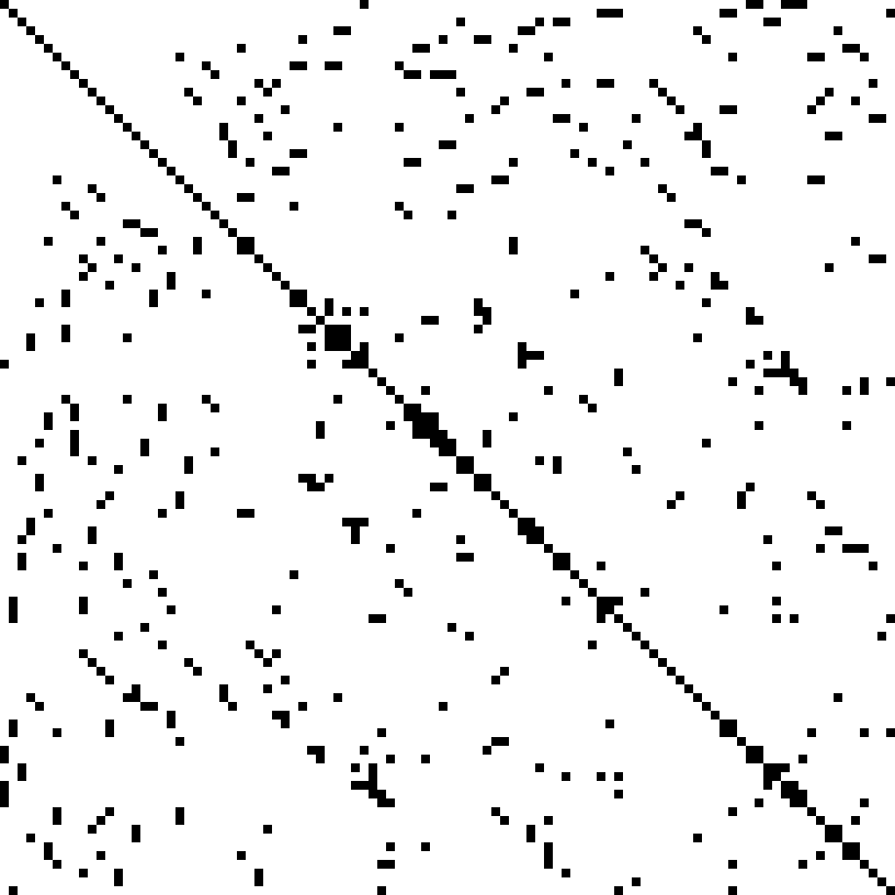 # [Source](https://commons.wikimedia.org/w/index.php?curid=2245335)
#
# There are the most common sparse storage formats:
# - coordinate-wise (scipy calls COO)
# - compressed sparse row (CSR)
# - compressed sparse column (CSC)
#
# Let's walk through [these examples](http://www.mathcs.emory.edu/~cheung/Courses/561/Syllabus/3-C/sparse.html)
#
# There are actually [many more formats](http://www.cs.colostate.edu/~mcrob/toolbox/c++/sparseMatrix/sparse_matrix_compression.html) as well.
#
# A class of matrices (e.g, diagonal) is generally called sparse if the number of non-zero elements is proportional to the number of rows (or columns) instead of being proportional to the product rows x columns.
#
# **Scipy Implementation**
#
# From the [Scipy Sparse Matrix Documentation](https://docs.scipy.org/doc/scipy-0.18.1/reference/sparse.html)
#
# - To construct a matrix efficiently, use either dok_matrix or lil_matrix. The lil_matrix class supports basic slicing and fancy indexing with a similar syntax to NumPy arrays. As illustrated below, the COO format may also be used to efficiently construct matrices
# - To perform manipulations such as multiplication or inversion, first convert the matrix to either CSC or CSR format.
# - All conversions among the CSR, CSC, and COO formats are efficient, linear-time operations.
# ## Today: CT scans
# ["Can Maths really save your life? Of course it can!!"](https://plus.maths.org/content/saving-lives-mathematics-tomography) (lovely article)
#
#
# [Source](https://commons.wikimedia.org/w/index.php?curid=2245335)
#
# There are the most common sparse storage formats:
# - coordinate-wise (scipy calls COO)
# - compressed sparse row (CSR)
# - compressed sparse column (CSC)
#
# Let's walk through [these examples](http://www.mathcs.emory.edu/~cheung/Courses/561/Syllabus/3-C/sparse.html)
#
# There are actually [many more formats](http://www.cs.colostate.edu/~mcrob/toolbox/c++/sparseMatrix/sparse_matrix_compression.html) as well.
#
# A class of matrices (e.g, diagonal) is generally called sparse if the number of non-zero elements is proportional to the number of rows (or columns) instead of being proportional to the product rows x columns.
#
# **Scipy Implementation**
#
# From the [Scipy Sparse Matrix Documentation](https://docs.scipy.org/doc/scipy-0.18.1/reference/sparse.html)
#
# - To construct a matrix efficiently, use either dok_matrix or lil_matrix. The lil_matrix class supports basic slicing and fancy indexing with a similar syntax to NumPy arrays. As illustrated below, the COO format may also be used to efficiently construct matrices
# - To perform manipulations such as multiplication or inversion, first convert the matrix to either CSC or CSR format.
# - All conversions among the CSR, CSC, and COO formats are efficient, linear-time operations.
# ## Today: CT scans
# ["Can Maths really save your life? Of course it can!!"](https://plus.maths.org/content/saving-lives-mathematics-tomography) (lovely article)
#
#  #
# (CAT and CT scan refer to the [same procedure](http://blog.cincinnatichildrens.org/radiology/whats-the-difference-between-a-cat-scan-and-a-ct-scan/). CT scan is the more modern term)
#
# This lesson is based off the Scikit-Learn example [Compressive sensing: tomography reconstruction with L1 prior (Lasso)](http://scikit-learn.org/stable/auto_examples/applications/plot_tomography_l1_reconstruction.html)
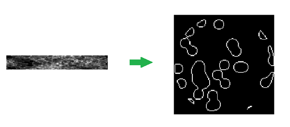
# #### Our goal today
# Take the readings from a CT scan and construct what the original looks like.
#
#
#
# (CAT and CT scan refer to the [same procedure](http://blog.cincinnatichildrens.org/radiology/whats-the-difference-between-a-cat-scan-and-a-ct-scan/). CT scan is the more modern term)
#
# This lesson is based off the Scikit-Learn example [Compressive sensing: tomography reconstruction with L1 prior (Lasso)](http://scikit-learn.org/stable/auto_examples/applications/plot_tomography_l1_reconstruction.html)
# #### Our goal today
# Take the readings from a CT scan and construct what the original looks like.
#
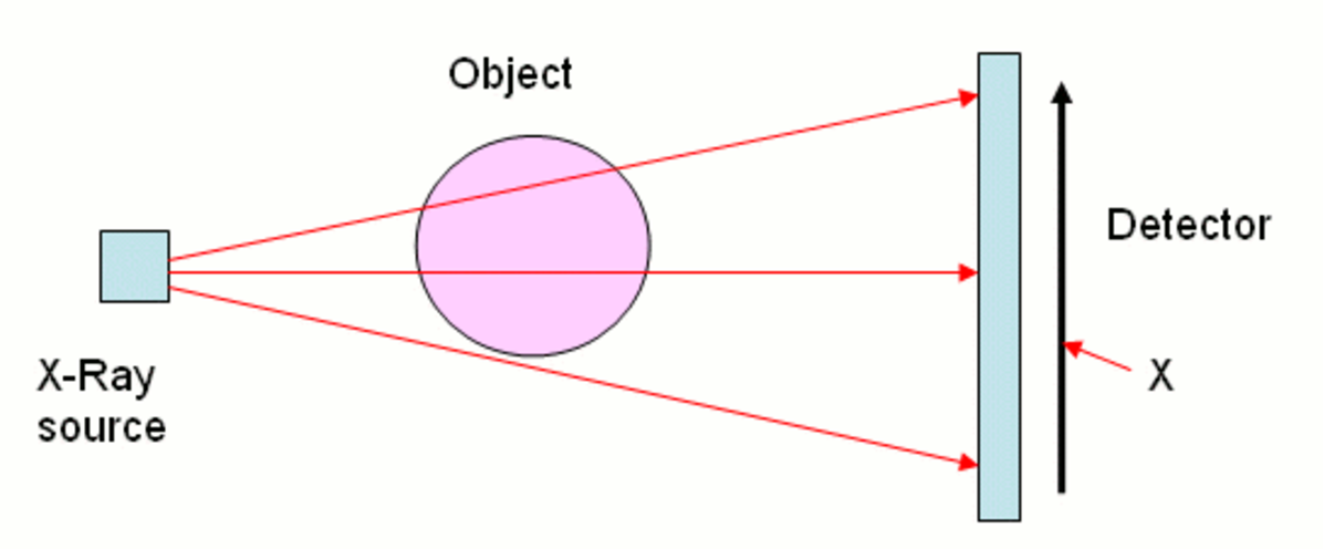
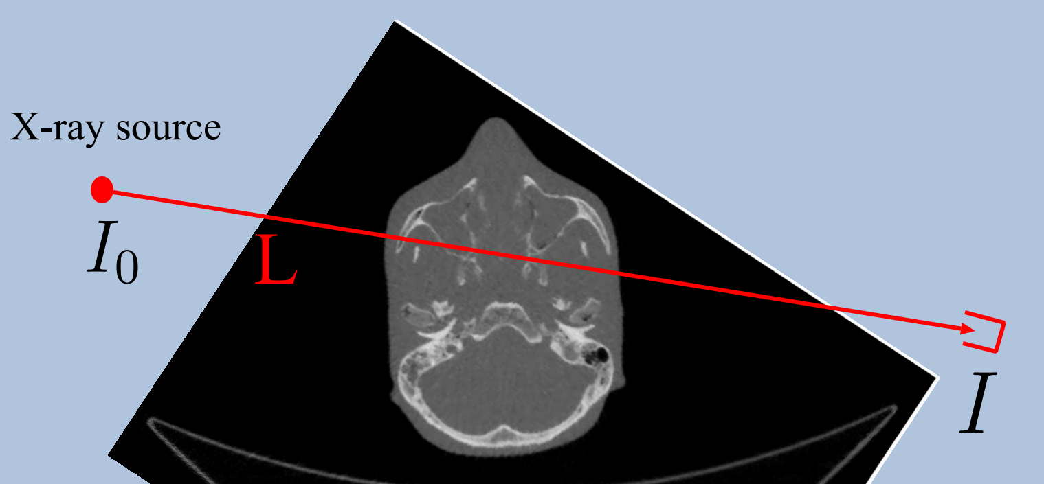
#  # For each x-ray (at a particular position and particular angle), we get a single measurement. We need to construct the original picture just from these measurements. Also, we don't want the patient to experience a ton of radiation, so we are gathering less data than the area of the picture.
#
#
# For each x-ray (at a particular position and particular angle), we get a single measurement. We need to construct the original picture just from these measurements. Also, we don't want the patient to experience a ton of radiation, so we are gathering less data than the area of the picture.
#
#  # ### Review
# In the previous lesson, we used Robust PCA for background removal of a surveillance video. We saw that this could be written as the optimization problem:
#
# $$ minimize\; \lVert L \rVert_* + \lambda\lVert S \rVert_1 \\ subject\;to\; L + S = M$$
#
# **Question**: Do you remember what is special about the L1 norm?
# #### Today
# We will see that:
#
#
# ### Review
# In the previous lesson, we used Robust PCA for background removal of a surveillance video. We saw that this could be written as the optimization problem:
#
# $$ minimize\; \lVert L \rVert_* + \lambda\lVert S \rVert_1 \\ subject\;to\; L + S = M$$
#
# **Question**: Do you remember what is special about the L1 norm?
# #### Today
# We will see that:
#
#  #
# Resources:
# [Compressed Sensing](https://people.csail.mit.edu/indyk/princeton.pdf)
#
#
#
# Resources:
# [Compressed Sensing](https://people.csail.mit.edu/indyk/princeton.pdf)
#
#  #
# [Source](https://www.fields.utoronto.ca/programs/scientific/10-11/medimaging/presentations/Plenary_Sidky.pdf)
# ### Imports
# In[1]:
get_ipython().run_line_magic('matplotlib', 'inline')
import numpy as np, matplotlib.pyplot as plt, math
from scipy import ndimage, sparse
# In[2]:
np.set_printoptions(suppress=True)
# ## Generate Data
# ### Intro
# We will use generated data today (not real CT scans). There is some interesting numpy and linear algebra involved in generating the data, and we will return to that later.
#
# Code is from this Scikit-Learn example [Compressive sensing: tomography reconstruction with L1 prior (Lasso)](http://scikit-learn.org/stable/auto_examples/applications/plot_tomography_l1_reconstruction.html)
# ### Generate pictures
# In[3]:
def generate_synthetic_data():
rs = np.random.RandomState(0)
n_pts = 36
x, y = np.ogrid[0:l, 0:l]
mask_outer = (x - l / 2) ** 2 + (y - l / 2) ** 2 < (l / 2) ** 2
mx,my = rs.randint(0, l, (2,n_pts))
mask = np.zeros((l, l))
mask[mx,my] = 1
mask = ndimage.gaussian_filter(mask, sigma=l / n_pts)
res = (mask > mask.mean()) & mask_outer
return res ^ ndimage.binary_erosion(res)
# In[208]:
l = 128
data = generate_synthetic_data()
# In[209]:
plt.figure(figsize=(5,5))
plt.imshow(data, cmap=plt.cm.gray);
# #### What generate_synthetic_data() is doing
# In[155]:
l=8; n_pts=5
rs = np.random.RandomState(0)
# In[156]:
x, y = np.ogrid[0:l, 0:l]; x,y
# In[170]:
x + y
# In[157]:
(x - l/2) ** 2
# In[59]:
(x - l/2) ** 2 + (y - l/2) ** 2
# In[60]:
mask_outer = (x - l/2) ** 2 + (y - l/2) ** 2 < (l/2) ** 2; mask_outer
# In[61]:
plt.imshow(mask_outer, cmap='gray')
# In[62]:
mask = np.zeros((l, l))
mx,my = rs.randint(0, l, (2,n_pts))
mask[mx,my] = 1; mask
# In[63]:
plt.imshow(mask, cmap='gray')
# In[64]:
mask = ndimage.gaussian_filter(mask, sigma=l / n_pts)
# In[65]:
plt.imshow(mask, cmap='gray')
# In[66]:
res = np.logical_and(mask > mask.mean(), mask_outer)
plt.imshow(res, cmap='gray');
# In[67]:
plt.imshow(ndimage.binary_erosion(res), cmap='gray');
# In[68]:
plt.imshow(res ^ ndimage.binary_erosion(res), cmap='gray');
# ### Generate Projections
# #### Code
# In[72]:
def _weights(x, dx=1, orig=0):
x = np.ravel(x)
floor_x = np.floor((x - orig) / dx)
alpha = (x - orig - floor_x * dx) / dx
return np.hstack((floor_x, floor_x + 1)), np.hstack((1 - alpha, alpha))
def _generate_center_coordinates(l_x):
X, Y = np.mgrid[:l_x, :l_x].astype(np.float64)
center = l_x / 2.
X += 0.5 - center
Y += 0.5 - center
return X, Y
# In[73]:
def build_projection_operator(l_x, n_dir):
X, Y = _generate_center_coordinates(l_x)
angles = np.linspace(0, np.pi, n_dir, endpoint=False)
data_inds, weights, camera_inds = [], [], []
data_unravel_indices = np.arange(l_x ** 2)
data_unravel_indices = np.hstack((data_unravel_indices,
data_unravel_indices))
for i, angle in enumerate(angles):
Xrot = np.cos(angle) * X - np.sin(angle) * Y
inds, w = _weights(Xrot, dx=1, orig=X.min())
mask = (inds >= 0) & (inds < l_x)
weights += list(w[mask])
camera_inds += list(inds[mask] + i * l_x)
data_inds += list(data_unravel_indices[mask])
proj_operator = sparse.coo_matrix((weights, (camera_inds, data_inds)))
return proj_operator
# #### Projection operator
# In[210]:
l = 128
# In[211]:
proj_operator = build_projection_operator(l, l // 7)
# In[212]:
proj_operator
# dimensions: angles (l//7), positions (l), image for each (l x l)
# In[213]:
proj_t = np.reshape(proj_operator.todense().A, (l//7,l,l,l))
# The first coordinate refers to the angle of the line, and the second coordinate refers to the location of the line.
# The lines for the angle indexed with 3:
# In[214]:
plt.imshow(proj_t[3,0], cmap='gray');
# In[215]:
plt.imshow(proj_t[3,1], cmap='gray');
# In[216]:
plt.imshow(proj_t[3,2], cmap='gray');
# In[217]:
plt.imshow(proj_t[3,40], cmap='gray');
# Other lines at vertical location 40:
# In[218]:
plt.imshow(proj_t[4,40], cmap='gray');
# In[219]:
plt.imshow(proj_t[15,40], cmap='gray');
# In[220]:
plt.imshow(proj_t[17,40], cmap='gray');
# #### Intersection between x-rays and data
# Next, we want to see how the line intersects with our data. Remember, this is what the data looks like:
# In[221]:
plt.figure(figsize=(5,5))
plt.imshow(data, cmap=plt.cm.gray)
plt.axis('off')
plt.savefig("images/data.png")
# In[222]:
proj = proj_operator @ data.ravel()[:, np.newaxis]
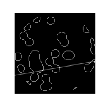
# An x-ray at angle 17, location 40 passing through the data:
# In[223]:
plt.figure(figsize=(5,5))
plt.imshow(data + proj_t[17,40], cmap=plt.cm.gray)
plt.axis('off')
plt.savefig("images/data_xray.png")
# Where they intersect:
# In[224]:
both = data + proj_t[17,40]
plt.imshow((both > 1.1).astype(int), cmap=plt.cm.gray);
# The intensity of an x-ray at angle 17, location 40 passing through the data:
# In[225]:
np.resize(proj, (l//7,l))[17,40]
# The intensity of an x-ray at angle 3, location 14 passing through the data:
# In[226]:
plt.imshow(data + proj_t[3,14], cmap=plt.cm.gray);
# Where they intersect:
# In[227]:
both = data + proj_t[3,14]
plt.imshow((both > 1.1).astype(int), cmap=plt.cm.gray);
# The measurement from the CT scan would be a small number here:
# In[228]:
np.resize(proj, (l//7,l))[3,14]
# In[229]:
proj += 0.15 * np.random.randn(*proj.shape)
# #### About *args
# In[230]:
a = [1,2,3]
b= [4,5,6]
# In[231]:
c = list(zip(a, b))
# In[232]:
c
# In[233]:
list(zip(*c))
# ### The Projection (CT readings)
# In[234]:
plt.figure(figsize=(7,7))
plt.imshow(np.resize(proj, (l//7,l)), cmap='gray')
plt.axis('off')
plt.savefig("images/proj.png")
# ## Regresssion
# Now we will try to recover the data just from the projections (the measurements of the CT scan)
# #### Linear Regression: $Ax = b$
# Our matrix $A$ is the projection operator. This was our 4d matrix above (angle, location, x, y) of the different x-rays:
# In[203]:
plt.figure(figsize=(12,12))
plt.title("A: Projection Operator")
plt.imshow(proj_operator.todense().A, cmap='gray')
# We are solving for $x$, the original data. We (un)ravel the 2D data into a single column.
# In[202]:
plt.figure(figsize=(5,5))
plt.title("x: Image")
plt.imshow(data, cmap='gray')
plt.figure(figsize=(4,12))
# I am tiling the column so that it's easier to see
plt.imshow(np.tile(data.ravel(), (80,1)).T, cmap='gray')
# Our vector $b$ is the (un)raveled matrix of measurements:
# In[238]:
plt.figure(figsize=(8,8))
plt.imshow(np.resize(proj, (l//7,l)), cmap='gray')
plt.figure(figsize=(10,10))
plt.imshow(np.tile(proj.ravel(), (20,1)).T, cmap='gray')
# #### Scikit Learn Linear Regression
# In[84]:
from sklearn.linear_model import Lasso
from sklearn.linear_model import Ridge
# In[126]:
# Reconstruction with L2 (Ridge) penalization
rgr_ridge = Ridge(alpha=0.2)
rgr_ridge.fit(proj_operator, proj.ravel())
rec_l2 = rgr_ridge.coef_.reshape(l, l)
plt.imshow(rec_l2, cmap='gray')
# In[179]:
18*128
# In[ ]:
18 x 128 x 128 x 128
# In[178]:
proj_operator.shape
# In[87]:
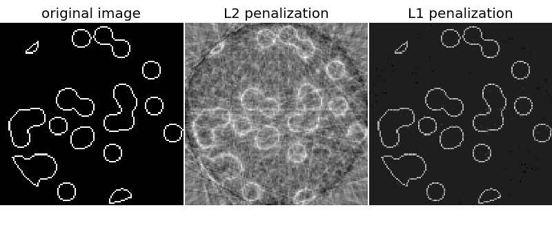
# Reconstruction with L1 (Lasso) penalization
# the best value of alpha was determined using cross validation
# with LassoCV
rgr_lasso = Lasso(alpha=0.001)
rgr_lasso.fit(proj_operator, proj.ravel())
rec_l1 = rgr_lasso.coef_.reshape(l, l)
plt.imshow(rec_l1, cmap='gray')
# The L1 penalty works significantly better than the L2 penalty here!
#
# [Source](https://www.fields.utoronto.ca/programs/scientific/10-11/medimaging/presentations/Plenary_Sidky.pdf)
# ### Imports
# In[1]:
get_ipython().run_line_magic('matplotlib', 'inline')
import numpy as np, matplotlib.pyplot as plt, math
from scipy import ndimage, sparse
# In[2]:
np.set_printoptions(suppress=True)
# ## Generate Data
# ### Intro
# We will use generated data today (not real CT scans). There is some interesting numpy and linear algebra involved in generating the data, and we will return to that later.
#
# Code is from this Scikit-Learn example [Compressive sensing: tomography reconstruction with L1 prior (Lasso)](http://scikit-learn.org/stable/auto_examples/applications/plot_tomography_l1_reconstruction.html)
# ### Generate pictures
# In[3]:
def generate_synthetic_data():
rs = np.random.RandomState(0)
n_pts = 36
x, y = np.ogrid[0:l, 0:l]
mask_outer = (x - l / 2) ** 2 + (y - l / 2) ** 2 < (l / 2) ** 2
mx,my = rs.randint(0, l, (2,n_pts))
mask = np.zeros((l, l))
mask[mx,my] = 1
mask = ndimage.gaussian_filter(mask, sigma=l / n_pts)
res = (mask > mask.mean()) & mask_outer
return res ^ ndimage.binary_erosion(res)
# In[208]:
l = 128
data = generate_synthetic_data()
# In[209]:
plt.figure(figsize=(5,5))
plt.imshow(data, cmap=plt.cm.gray);
# #### What generate_synthetic_data() is doing
# In[155]:
l=8; n_pts=5
rs = np.random.RandomState(0)
# In[156]:
x, y = np.ogrid[0:l, 0:l]; x,y
# In[170]:
x + y
# In[157]:
(x - l/2) ** 2
# In[59]:
(x - l/2) ** 2 + (y - l/2) ** 2
# In[60]:
mask_outer = (x - l/2) ** 2 + (y - l/2) ** 2 < (l/2) ** 2; mask_outer
# In[61]:
plt.imshow(mask_outer, cmap='gray')
# In[62]:
mask = np.zeros((l, l))
mx,my = rs.randint(0, l, (2,n_pts))
mask[mx,my] = 1; mask
# In[63]:
plt.imshow(mask, cmap='gray')
# In[64]:
mask = ndimage.gaussian_filter(mask, sigma=l / n_pts)
# In[65]:
plt.imshow(mask, cmap='gray')
# In[66]:
res = np.logical_and(mask > mask.mean(), mask_outer)
plt.imshow(res, cmap='gray');
# In[67]:
plt.imshow(ndimage.binary_erosion(res), cmap='gray');
# In[68]:
plt.imshow(res ^ ndimage.binary_erosion(res), cmap='gray');
# ### Generate Projections
# #### Code
# In[72]:
def _weights(x, dx=1, orig=0):
x = np.ravel(x)
floor_x = np.floor((x - orig) / dx)
alpha = (x - orig - floor_x * dx) / dx
return np.hstack((floor_x, floor_x + 1)), np.hstack((1 - alpha, alpha))
def _generate_center_coordinates(l_x):
X, Y = np.mgrid[:l_x, :l_x].astype(np.float64)
center = l_x / 2.
X += 0.5 - center
Y += 0.5 - center
return X, Y
# In[73]:
def build_projection_operator(l_x, n_dir):
X, Y = _generate_center_coordinates(l_x)
angles = np.linspace(0, np.pi, n_dir, endpoint=False)
data_inds, weights, camera_inds = [], [], []
data_unravel_indices = np.arange(l_x ** 2)
data_unravel_indices = np.hstack((data_unravel_indices,
data_unravel_indices))
for i, angle in enumerate(angles):
Xrot = np.cos(angle) * X - np.sin(angle) * Y
inds, w = _weights(Xrot, dx=1, orig=X.min())
mask = (inds >= 0) & (inds < l_x)
weights += list(w[mask])
camera_inds += list(inds[mask] + i * l_x)
data_inds += list(data_unravel_indices[mask])
proj_operator = sparse.coo_matrix((weights, (camera_inds, data_inds)))
return proj_operator
# #### Projection operator
# In[210]:
l = 128
# In[211]:
proj_operator = build_projection_operator(l, l // 7)
# In[212]:
proj_operator
# dimensions: angles (l//7), positions (l), image for each (l x l)
# In[213]:
proj_t = np.reshape(proj_operator.todense().A, (l//7,l,l,l))
# The first coordinate refers to the angle of the line, and the second coordinate refers to the location of the line.
# The lines for the angle indexed with 3:
# In[214]:
plt.imshow(proj_t[3,0], cmap='gray');
# In[215]:
plt.imshow(proj_t[3,1], cmap='gray');
# In[216]:
plt.imshow(proj_t[3,2], cmap='gray');
# In[217]:
plt.imshow(proj_t[3,40], cmap='gray');
# Other lines at vertical location 40:
# In[218]:
plt.imshow(proj_t[4,40], cmap='gray');
# In[219]:
plt.imshow(proj_t[15,40], cmap='gray');
# In[220]:
plt.imshow(proj_t[17,40], cmap='gray');
# #### Intersection between x-rays and data
# Next, we want to see how the line intersects with our data. Remember, this is what the data looks like:
# In[221]:
plt.figure(figsize=(5,5))
plt.imshow(data, cmap=plt.cm.gray)
plt.axis('off')
plt.savefig("images/data.png")
# In[222]:
proj = proj_operator @ data.ravel()[:, np.newaxis]
# An x-ray at angle 17, location 40 passing through the data:
# In[223]:
plt.figure(figsize=(5,5))
plt.imshow(data + proj_t[17,40], cmap=plt.cm.gray)
plt.axis('off')
plt.savefig("images/data_xray.png")
# Where they intersect:
# In[224]:
both = data + proj_t[17,40]
plt.imshow((both > 1.1).astype(int), cmap=plt.cm.gray);
# The intensity of an x-ray at angle 17, location 40 passing through the data:
# In[225]:
np.resize(proj, (l//7,l))[17,40]
# The intensity of an x-ray at angle 3, location 14 passing through the data:
# In[226]:
plt.imshow(data + proj_t[3,14], cmap=plt.cm.gray);
# Where they intersect:
# In[227]:
both = data + proj_t[3,14]
plt.imshow((both > 1.1).astype(int), cmap=plt.cm.gray);
# The measurement from the CT scan would be a small number here:
# In[228]:
np.resize(proj, (l//7,l))[3,14]
# In[229]:
proj += 0.15 * np.random.randn(*proj.shape)
# #### About *args
# In[230]:
a = [1,2,3]
b= [4,5,6]
# In[231]:
c = list(zip(a, b))
# In[232]:
c
# In[233]:
list(zip(*c))
# ### The Projection (CT readings)
# In[234]:
plt.figure(figsize=(7,7))
plt.imshow(np.resize(proj, (l//7,l)), cmap='gray')
plt.axis('off')
plt.savefig("images/proj.png")
# ## Regresssion
# Now we will try to recover the data just from the projections (the measurements of the CT scan)
# #### Linear Regression: $Ax = b$
# Our matrix $A$ is the projection operator. This was our 4d matrix above (angle, location, x, y) of the different x-rays:
# In[203]:
plt.figure(figsize=(12,12))
plt.title("A: Projection Operator")
plt.imshow(proj_operator.todense().A, cmap='gray')
# We are solving for $x$, the original data. We (un)ravel the 2D data into a single column.
# In[202]:
plt.figure(figsize=(5,5))
plt.title("x: Image")
plt.imshow(data, cmap='gray')
plt.figure(figsize=(4,12))
# I am tiling the column so that it's easier to see
plt.imshow(np.tile(data.ravel(), (80,1)).T, cmap='gray')
# Our vector $b$ is the (un)raveled matrix of measurements:
# In[238]:
plt.figure(figsize=(8,8))
plt.imshow(np.resize(proj, (l//7,l)), cmap='gray')
plt.figure(figsize=(10,10))
plt.imshow(np.tile(proj.ravel(), (20,1)).T, cmap='gray')
# #### Scikit Learn Linear Regression
# In[84]:
from sklearn.linear_model import Lasso
from sklearn.linear_model import Ridge
# In[126]:
# Reconstruction with L2 (Ridge) penalization
rgr_ridge = Ridge(alpha=0.2)
rgr_ridge.fit(proj_operator, proj.ravel())
rec_l2 = rgr_ridge.coef_.reshape(l, l)
plt.imshow(rec_l2, cmap='gray')
# In[179]:
18*128
# In[ ]:
18 x 128 x 128 x 128
# In[178]:
proj_operator.shape
# In[87]:
# Reconstruction with L1 (Lasso) penalization
# the best value of alpha was determined using cross validation
# with LassoCV
rgr_lasso = Lasso(alpha=0.001)
rgr_lasso.fit(proj_operator, proj.ravel())
rec_l1 = rgr_lasso.coef_.reshape(l, l)
plt.imshow(rec_l1, cmap='gray')
# The L1 penalty works significantly better than the L2 penalty here!