#!/usr/bin/env python # coding: utf-8 # # Frame of reference # # # > Marcos Duarte, Renato Naville Watanabe # > [Laboratory of Biomechanics and Motor Control](https://bmclab.pesquisa.ufabc.edu.br/) # > Federal University of ABC, Brazil #

1 Frame of reference for human motion analysis
2 Cartesian coordinate system
- 2.1 Standardizations in movement analysis
3 Determination of a coordinate system
4 Further reading
5 Video lectures on the Internet
6 Problems
7 References

# Motion (a change of position in space with respect to time) is not an absolute concept; a reference is needed to describe the motion of the object in relation to this reference. Likewise, the state of such reference cannot be absolute in space and so motion is relative. # A [frame of reference](http://en.wikipedia.org/wiki/Frame_of_reference) is the place with respect to we choose to describe the motion of an object. In this reference frame, we define a [coordinate system](http://en.wikipedia.org/wiki/Coordinate_system) (a set of axes) within which we measure the motion of an object (but frame of reference and coordinate system are often used interchangeably). # # Often, the choice of reference frame and coordinate system is made by convenience. However, there is an important distinction between reference frames when we deal with the dynamics of motion, where we are interested to understand the forces related to the motion of the object. In dynamics, we refer to [inertial frame of reference](http://en.wikipedia.org/wiki/Inertial_frame_of_reference) (a.k.a., Galilean reference frame) when the Newton's laws of motion in their simple form are valid in this frame and to non-inertial frame of reference when the Newton's laws in their simple form are not valid (in such reference frame, fictitious accelerations/forces appear). An inertial reference frame is at rest or moves at constant speed (because there is no absolute rest!), whereas a non-inertial reference frame is under acceleration (with respect to an inertial reference frame). # # The concept of frame of reference has changed drastically since Aristotle, Galileo, Newton, and Einstein. To read more about that and its philosophical implications, see [Space and Time: Inertial Frames](http://plato.stanford.edu/entries/spacetime-iframes/). # ## Frame of reference for human motion analysis # # In anatomy, we use a simplified reference frame composed by perpendicular planes to provide a standard reference for qualitatively describing the structures and movements of the human body, as shown in the next figure. # #

*Figure. Anatomical body position and body planes (image from Wikipedia).*

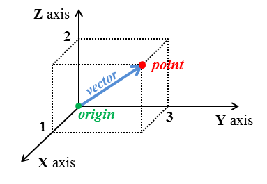
# ## Cartesian coordinate system # # As we perceive the surrounding space as three-dimensional, a convenient coordinate system is the [Cartesian coordinate system](http://en.wikipedia.org/wiki/Cartesian_coordinate_system) in the [Euclidean space](http://en.wikipedia.org/wiki/Euclidean_space) with three orthogonal axes as shown below. The axes directions are commonly defined by the [right-hand rule](http://en.wikipedia.org/wiki/Right-hand_rule) and attributed the letters X, Y, Z. The orthogonality of the Cartesian coordinate system is convenient for its use in classical mechanics, most of the times the structure of space is assumed having the [Euclidean geometry](http://en.wikipedia.org/wiki/Euclidean_geometry) and as consequence, the motion in different directions are independent of each other. # #

*Figure. A point in three-dimensional Euclidean space described in a Cartesian coordinate system.*

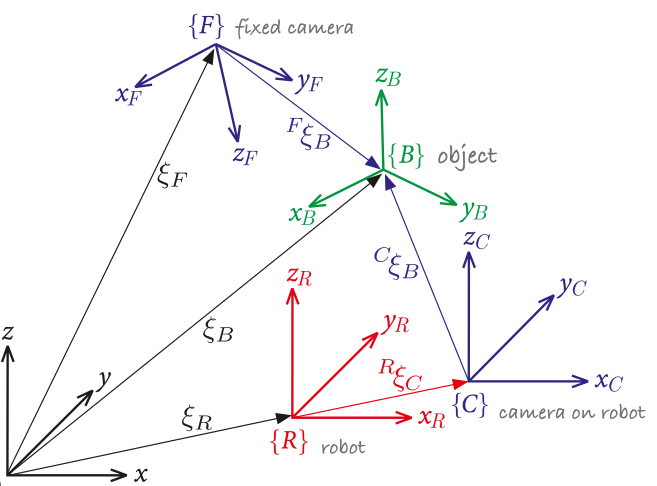
# ### Standardizations in movement analysis # # The concept of reference frame in Biomechanics and motor control is very important and central to the understanding of human motion. For example, do we see, plan and control the movement of our hand with respect to reference frames within our body or in the environment we move? Or a combination of both? # The figure below, although derived for a robotic system, illustrates well the concept that we might have to deal with multiple coordinate systems. # #

*Figure. Multiple coordinate systems for use in robots (figure from Corke (2017)).*

# # For three-dimensional motion analysis in Biomechanics, we may use several different references frames for convenience and refer to them as global, laboratory, local, anatomical, or technical reference frames or coordinate systems (we will study this later). # There has been proposed different standardizations on how to define frame of references for the main segments and joints of the human body. For instance, the International Society of Biomechanics has a [page listing standardization proposals](https://isbweb.org/activities/standards) by its standardization committee and subcommittees: # In[1]: from IPython.display import IFrame IFrame('https://isbweb.org/activities/standards', width='100%', height=400) # Another initiative for the standardization of references frames is from the [Virtual Animation of the Kinematics of the Human for Industrial, Educational and Research Purposes (VAKHUM)](https://github.com/BMClab/BMC/blob/master/courses/refs/VAKHUM.pdf) project. # ## Determination of a coordinate system # # In Biomechanics, we may use different coordinate systems for convenience and refer to them as global, laboratory, local, anatomical, or technical reference frames or coordinate systems. For example, in a standard gait analysis, we define a global or laboratory coordinate system and a different coordinate system for each segment of the body to be able to describe the motion of a segment in relation to anatomical axes of another segment. To define this anatomical coordinate system, we need to place markers on anatomical landmarks on each segment. We also may use other markers (technical markers) on the segment to improve the motion analysis and then we will also have to define a technical coordinate system for each segment. 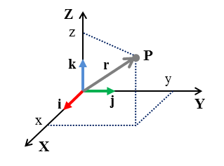# # As we perceive the surrounding space as three-dimensional, a convenient coordinate system to use is the [Cartesian coordinate system](http://en.wikipedia.org/wiki/Cartesian_coordinate_system) with three orthogonal axes in the [Euclidean space](http://en.wikipedia.org/wiki/Euclidean_space). From [linear algebra](http://en.wikipedia.org/wiki/Linear_algebra), a set of unit linearly independent vectors (orthogonal in the Euclidean space and each with norm (length) equals to one) that can represent any vector via [linear combination](http://en.wikipedia.org/wiki/Linear_combination) is called a basis (or orthonormal basis). The figure below shows a point and its position vector in the Cartesian coordinate system and the corresponding versors (unit vectors) of the basis for this coordinate system. See the notebook [Scalar and vector](http://nbviewer.ipython.org/github/demotu/BMC/blob/master/notebooks/ScalarVector.ipynb) for a description on vectors. # #

Figure. Representation of a point P and its position vector $\overrightarrow{\mathbf{r}}$ in a Cartesian coordinate system. The versors $\hat{\mathbf{i}}, \hat{\mathbf{j}}, \hat{\mathbf{k}}$ form a basis for this coordinate system and are usually represented in the color sequence RGB (red, green, blue) for easier visualization.

# # One can see that the versors of the basis shown in the figure above have the following coordinates in the Cartesian coordinate system: #
# # \begin{equation} # \hat{\mathbf{i}} = \begin{bmatrix}1\\0\\0 \end{bmatrix}, \quad \hat{\mathbf{j}} = \begin{bmatrix}0\\1\\0 \end{bmatrix}, \quad \hat{\mathbf{k}} = \begin{bmatrix} 0 \\ 0 \\ 1 \end{bmatrix} # \end{equation} # # # Using the notation described in the figure above, the position vector $\overrightarrow{\mathbf{r}}$ (or the point $\overrightarrow{\mathbf{P}}$) can be expressed as: #
# # \begin{equation} # \overrightarrow{\mathbf{r}} = x\hat{\mathbf{i}} + y\hat{\mathbf{j}} + z\hat{\mathbf{k}} # \end{equation} # # ### Definition of a basis # # The mathematical problem of determination of a coordinate system is to find a basis and an origin for it (a basis is only a set of vectors, with no origin). There are different methods to calculate a basis given a set of points (coordinates), for example, one can use the scalar product or the cross product for this problem. # ### Using the cross product # # Let's now define a basis using a common method in motion analysis (employing the cross product): # Given the coordinates of three noncollinear points in 3D space (points that do not all lie on the same line), $\overrightarrow{\mathbf{m}}_1, \overrightarrow{\mathbf{m}}_2, \overrightarrow{\mathbf{m}}_3$, which would represent the positions of markers captured from a motion analysis session, a basis can be found following these steps: # # 1. First axis, $\overrightarrow{\mathbf{v}}_1$, the vector $\overrightarrow{\mathbf{m}}_2-\overrightarrow{\mathbf{m}}_1$ (or any other vector difference); # # 2. Second axis, $\overrightarrow{\mathbf{v}}_2$, the cross or vector product between the vectors $\overrightarrow{\mathbf{v}}_1$ and $\overrightarrow{\mathbf{m}}_3-\overrightarrow{\mathbf{m}}_1$ (or $\overrightarrow{\mathbf{m}}_3-\overrightarrow{\mathbf{m}}_2$); # # 3. Third axis, $\overrightarrow{\mathbf{v}}_3$, the cross product between the vectors $\overrightarrow{\mathbf{v}}_1$ and $\overrightarrow{\mathbf{v}}_2$; and # # 4. Make all vectors to have norm 1 dividing each vector by its norm. # The positions of the points used to construct a coordinate system have, by definition, to be specified in relation to an already existing coordinate system. In motion analysis, this coordinate system is the coordinate system from the motion capture system and it is established in the calibration phase. In this phase, the positions of markers placed on an object with perpendicular axes and known distances between the markers are captured and used as the reference (laboratory) coordinate system. # For example, given the positions $\overrightarrow{\mathbf{m}}_1 = [1,2,5], \overrightarrow{\mathbf{m}}_2 = [2,3,3], \overrightarrow{\mathbf{m}}_3 = [4,0,2]$, a basis can be found with: # In[2]: import numpy as np m1 = np.array([1, 2, 5]) m2 = np.array([2, 3, 3]) m3 = np.array([4, 0, 2]) v1 = m2 - m1 # first axis v2 = np.cross(v1, m3 - m1) # second axis v3 = np.cross(v1, v2) # third axis # Vector normalization e1 = v1/np.linalg.norm(v1) e2 = v2/np.linalg.norm(v2) e3 = v3/np.linalg.norm(v3) print('Versors:', '\ne1 =', e1, '\ne2 =', e2, '\ne3 =', e3) print('\nNorm of each versor:', '\n||e1|| =', np.linalg.norm(e1), '\n||e2|| =', np.linalg.norm(e2), '\n||e3|| =', np.linalg.norm(e3)) print('\nTest of orthogonality (cross product between versors):', '\ne1 x e2:', np.linalg.norm(np.cross(e1, e2)), '\ne1 x e3:', np.linalg.norm(np.cross(e1, e3)), '\ne2 x e3:', np.linalg.norm(np.cross(e2, e3))) # Due to rounding errors ([see here](https://en.wikipedia.org/wiki/Round-off_error)) and to the imprecision of the computation with decimal floating-point numbers ([see here](http://docs.python.org/2/tutorial/floatingpoint.html)), the norms are not exactly equal to 1. # We could round the result if desired: # In[3]: print('\nTest of orthogonality (cross product between versors):', '\ne1 x e2:', np.linalg.norm(np.cross(e1, e2)).round(8), '\ne1 x e3:', np.linalg.norm(np.cross(e1, e3)).round(8), '\ne2 x e3:', np.linalg.norm(np.cross(e2, e3)).round(8)) # Or format the text representing the result: # In[4]: print('\nTest of orthogonality (cross product between versors):', f'\ne1 x e2: {np.linalg.norm(np.cross(e1, e2)):g}', f'\ne1 x e3: {np.linalg.norm(np.cross(e1, e3)):g}', f'\ne2 x e3: {np.linalg.norm(np.cross(e2, e3)):g}') # Where we used `f'{:.g}'` to format the number to a string ([see here](https://docs.python.org/dev/library/stdtypes.html#printf-style-string-formatting) and a [Python F-Strings Number Formatting Cheat Sheet](https://cheatography.com/brianallan/cheat-sheets/python-f-strings-number-formatting/)). # # For a permanent change, we could use the numpy settings for the representation of the decimal point precision with the function [`np.set_printoptions`](https://numpy.org/doc/stable/reference/generated/numpy.set_printoptions.html) but it only works for numpy arrays, not with numbers. Or use the IPython magic command [`%precision`](https://ipython.readthedocs.io/en/stable/interactive/magics.html#magic-precision), but in this case you can not use the function print for showing the result. # ### Coordinate system: origin and basis # # To define a coordinate system using the calculated basis, we also need to define an origin. In principle, we could use any point as origin, but if the calculated coordinate system should follow anatomical conventions, e.g., the coordinate system origin should be at a joint center, we will have to calculate the basis and origin according to standards used in motion analysis as discussed before. # # If the coordinate system is a technical basis and not anatomic-based, a common procedure in motion analysis is to define the origin for the coordinate system as the centroid (average) position among the markers at the reference frame. Using the average position across markers potentially reduces the effect of noise (for example, from soft tissue artifact) on the calculation. # # For the markers in the example above, the origin of the coordinate system will be: # In[5]: origin = np.mean((m1, m2, m3), axis=0) print('Origin: ', origin) # Let's plot the coordinate system and the basis using the custom Python function `CCS.py`. # We could copy and paste the content of the `CCS.py` here (and execute the cell) or we could load the function from a directory in the Google Drive, let's do that. First, create a folder "functions" and place the `CCS.py` file in it. # In[6]: if 'google.colab' in str(get_ipython()): # only if you are in Google Colab print('Google drive will be mounted.') print('Create folder "functions" and place functions in it.') from google.colab import drive drive.mount('/content/drive', force_remount=True) path2 = r'/content/drive/MyDrive/functions' else: path2 = r'./../functions' import sys sys.path.insert(1, path2) # add to pythonpath from CCS import CCS # In[7]: markers = np.vstack((m1, m2, m3)) basis = np.vstack((e1, e2, e3)) # #### Visualization of the coordinate system # # To have an interactive matplotlib plot we have to install the library `ipympl` and restart the Google Colab environment before using it for the first time. # In[8]: # to install ipympl in Google Colab (for interactive matplotlib) get_ipython().system('pip install -q ipympl') #

RESTART THE GOOGLE COLAB ENVIRONMENT AND RE-EXECUTE ALL CELLS BEFORE THIS POINT!

# In[9]: if 'google.colab' in str(get_ipython()): from google.colab import output output.enable_custom_widget_manager() # In[10]: get_ipython().run_line_magic('matplotlib', 'widget') CCS(xyz=[], Oijk=origin, ijk=basis, point=markers, vector=True); # ### Gram–Schmidt process # # Another classical procedure in mathematics, employing the scalar product, is known as the [Gram–Schmidt process](http://en.wikipedia.org/wiki/Gram%E2%80%93Schmidt_process). See the notebook [Scalar and Vector](http://nbviewer.jupyter.org/github/bmclab/BMC/blob/master/notebooks/ScalarVector.ipynb) for a demonstration of the Gram–Schmidt process and how to implement it in Python. # # The [Gram–Schmidt process](http://en.wikipedia.org/wiki/Gram%E2%80%93Schmidt_process) is a method for orthonormalizing (orthogonal unit versors) a set of vectors using the scalar product. The Gram–Schmidt process works for any number of vectors. # # For example, given three vectors, # $\overrightarrow{\mathbf{a}}, \overrightarrow{\mathbf{b}}, \overrightarrow{\mathbf{c}}$, in the 3D space, a basis $\{\hat{e}_a, \hat{e}_b, \hat{e}_c\}$ can be found using the Gram–Schmidt process by: # The first versor is in the # $\overrightarrow{\mathbf{a}}$ direction (or in the direction of any of the other vectors): #
# # \begin{equation} # \hat{e}_a = \frac{\overrightarrow{\mathbf{a}}}{||\overrightarrow{\mathbf{a}}||} # \end{equation} # # The second versor, orthogonal to $\hat{e}_a$, can be found considering we can express vector $\overrightarrow{\mathbf{b}}$ in terms of the $\hat{e}_a$ direction as: #
# # \begin{equation} # \overrightarrow{\mathbf{b}} = \overrightarrow{\mathbf{b}}^\| + \overrightarrow{\mathbf{b}}^\bot # \end{equation} # # # Then: # # # \begin{equation} # \overrightarrow{\mathbf{b}}^\bot = \overrightarrow{\mathbf{b}} - \overrightarrow{\mathbf{b}}^\| = \overrightarrow{\mathbf{b}} - (\overrightarrow{\mathbf{b}} \cdot \hat{e}_a ) \hat{e}_a # \end{equation} # # # Finally: # # # \begin{equation} # \hat{e}_b = \frac{\overrightarrow{\mathbf{b}}^\bot}{||\overrightarrow{\mathbf{b}}^\bot||} # \end{equation} # # The third versor, orthogonal to $\{\hat{e}_a, \hat{e}_b\}$, can be found expressing the vector $\overrightarrow{\mathbf{C}}$ in terms of $\hat{e}_a$ and $\hat{e}_b$ directions as: #
# # \begin{equation} # \overrightarrow{\mathbf{c}} = \overrightarrow{\mathbf{c}}^\| + \overrightarrow{\mathbf{c}}^\bot # \end{equation} # # # Then: # # \begin{equation} # \overrightarrow{\mathbf{c}}^\bot = \overrightarrow{\mathbf{c}} - \overrightarrow{\mathbf{c}}^\| # \end{equation} # # # Where: # # \begin{equation} # \overrightarrow{\mathbf{c}}^\| = (\overrightarrow{\mathbf{c}} \cdot \hat{e}_a ) \hat{e}_a + (\overrightarrow{\mathbf{c}} \cdot \hat{e}_b ) \hat{e}_b # \end{equation} # # # Finally: # # \begin{equation} # \hat{e}_c = \frac{\overrightarrow{\mathbf{c}}^\bot}{||\overrightarrow{\mathbf{c}}^\bot||} # \end{equation} # # And an animation of the Gram-Schmidt process being executed: # #

*Figure. The Gram-Schmidt process being executed on three vectors of a basis for R3 (image from Wikipedia).*

# Let's implement the Gram–Schmidt process in Python. # # For example, given the positions we seen before, $\overrightarrow{\mathbf{m}}_1 = [1,2,5], \overrightarrow{\mathbf{m}}_2 = [2,3,3], \overrightarrow{\mathbf{m}}_3 = [4,0,2]$, a basis can be found with: # The first versor is: # In[11]: ea = m1/np.linalg.norm(m1) print(ea) # The second versor is: # In[12]: eb = m2 - np.dot(m2, ea)*ea eb = eb/np.linalg.norm(eb) print(eb) # And the third version is: # In[13]: ec = m3 - np.dot(m3, ea)*ea - np.dot(m3, eb)*eb ec = ec/np.linalg.norm(ec) print(ec) # Let's check the orthonormality between these versors: # In[14]: print(" Versors:", "\nea =", ea, "\neb =", eb, "\nec =", ec) print( "\n Norm of each versor:", "\n ||ea|| =", np.linalg.norm(ea), "\n ||eb|| =", np.linalg.norm(eb), "\n ||ec|| =", np.linalg.norm(ec), ) print( "\n Test of orthogonality (scalar product between versors):", "\n ea . eb:", np.dot(ea, eb), "\n eb . ec:", np.dot(eb, ec), "\n ec . ea:", np.dot(ec, ea), ) # #### Visualization of the coordinate system # In[15]: # your turn ... # ## Further reading # # - [The right frame of reference makes it simple: An example of introductory mechanics supported by video analysis of motion](https://www.researchgate.net/publication/267761615_The_right_frame_of_reference_makes_it_simple_An_example_of_introductory_mechanics_supported_by_video_analysis_of_motion) # # ## Video lectures on the Internet # # - [Introduction to reference - Khan Academy](https://www.khanacademy.org/science/physics/one-dimensional-motion/displacement-velocity-time/v/introduction-to-reference-frames) # - [Introduction to orthonormal bases - Khan Academy](https://www.khanacademy.org/math/linear-algebra/alternate-bases/orthonormal-basis/v/linear-algebra-introduction-to-orthonormal-bases) # - [The Gram-Schmidt process - Khan Academy](https://www.khanacademy.org/math/linear-algebra/alternate-bases/orthonormal-basis/v/linear-algebra-the-gram-schmidt-process) # - [Biomechanics of Movement | Demo: Motion Capture Placement and Reference Frames](https://youtu.be/ctwoH59Obew) # ## Problems # # 1. Right now, how fast are you moving? In your answer, consider your motion in relation to Earth and in relation to Sun. # # 2. Go to the website [http://www.wisc-online.com/Objects/ViewObject.aspx?ID=AP15305](http://www.wisc-online.com/Objects/ViewObject.aspx?ID=AP15305) and complete the interactive lesson to learn about the anatomical terminology to describe relative position in the human body. # # 3. To learn more about Cartesian coordinate systems go to the website [http://www.mathsisfun.com/data/cartesian-coordinates.html](http://www.mathsisfun.com/data/cartesian-coordinates.html), study the material, and answer the 10 questions at the end. # # 4. Given the points in the 3D space, m1 = [2, 2, 0], m2 = [0, 1, 1], m3 = [1, 2, 0], find an orthonormal basis. # # 5. Determine if the following points form a basis in the 3D space, m1 = [2, 2, 0], m2 = [1, 1, 1], m3 = [1, 1, 0]. # # 6. Derive expressions for the three axes of the pelvic basis considering the convention of the [Virtual Animation of the Kinematics of the Human for Industrial, Educational and Research Purposes (VAKHUM)](https://github.com/BMClab/BMC/blob/master/courses/refs/VAKHUM.pdf) project (use RASIS, LASIS, RPSIS, and LPSIS as names for the pelvic anatomical landmarks and indicate the expression for each axis). # # 7. Determine the basis for the pelvis following the convention of the [Virtual Animation of the Kinematics of the Human for Industrial, Educational and Research Purposes (VAKHUM)](https://github.com/BMClab/BMC/blob/master/courses/refs/VAKHUM.pdf) project for the following anatomical landmark positions (units in meters): RASIS=[0.5, 0.8, 0.4], LASIS=[0.55, 0.78, 0.1], RPSIS=[0.3, 0.85, 0.2], LPSIS=[0.29, 0.78, 0.3]. # ## References # # - Corke P (2017) [Robotics, Vision and Control: Fundamental Algorithms in MATLAB](https://petercorke.com/RVC/). 2nd ed. Springer-Verlag Berlin. # - [Standards - International Society of Biomechanics](https://isbweb.org/activities/standards). # - Stanford Encyclopedia of Philosophy. [Space and Time: Inertial Frames](http://plato.stanford.edu/entries/spacetime-iframes/). # - [Virtual Animation of the Kinematics of the Human for Industrial, Educational and Research Purposes (VAKHUM)](https://github.com/BMClab/BMC/blob/master/courses/refs/VAKHUM.pdf).

Contents