#!/usr/bin/env python # coding: utf-8 #

# # Rigid-body transformations in a plane (2D) # # > Marcos Duarte, Renato Naville Watanabe # > [Laboratory of Biomechanics and Motor Control](https://bmclab.pesquisa.ufabc.edu.br) # > Federal University of ABC, Brazil #

# # ## Affine transformations # # Translation and rotation are two examples of [affine transformations](https://en.wikipedia.org/wiki/Affine_transformation). Affine transformations preserve straight lines, but not necessarily the distance between points. Other examples of affine transformations are scaling, shear, and reflection. The figure below illustrates different affine transformations in a plane. Note that a 3x3 matrix is shown on top of each transformation; these matrices are known as the transformation matrices and are the mathematical representation of the physical transformations. Next, we will study how to use this approach to describe the translation and rotation of a rigid-body. #
#

# ## Kinematics of a rigid body # The kinematics of a rigid body is completely described by its pose, i.e., its position and orientation in space (and the corresponding changes are translation and rotation). The translation and rotation of a rigid body are also known as rigid-body transformations (or simply, rigid transformations). # # Remember that in physics, a [rigid body](https://en.wikipedia.org/wiki/Rigid_body) is a model (an idealization) for a body in which deformation is neglected, i.e., the distance between every pair of points in the body is considered constant. Consequently, the position and orientation of a rigid body can be completely described by a corresponding coordinate system attached to it. For instance, two (or more) coordinate systems can be used to represent the same rigid body at two (or more) instants or two (or more) rigid bodies in space. # # Rigid-body transformations are used in motion analysis (e.g., of the human body) to describe the position and orientation of each segment (using a local (anatomical) coordinate system defined for each segment) in relation to a global coordinate system fixed at the laboratory. Furthermore, one can define an additional coordinate system called technical coordinate system also fixed at the rigid body but not based on anatomical landmarks. In this case, the position of the technical markers is first described in the laboratory coordinate system, and then the technical coordinate system is calculated to recreate the anatomical landmarks position in order to finally calculate the original anatomical coordinate system (and obtain its unknown position and orientation through time). # # In what follows, we will study rigid-body transformations by looking at the transformations between two coordinate systems. For simplicity, let's first analyze planar (two-dimensional) rigid-body transformations and later we will extend these concepts to three dimensions (where the study of rotations are more complicated). # ## Python setup # In[1]: import numpy as np np.set_printoptions(precision=4, suppress=True) # ## Translation # # In a two-dimensional space, two coordinates and one angle are sufficient to describe the pose of the rigid body, totalizing three degrees of freedom for a rigid body. Let's see first the transformation for translation, then for rotation, and combine them at last. 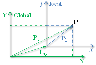# # A pure two-dimensional translation of a coordinate system in relation to other coordinate system and the representation of a point in these two coordinate systems are illustrated in the figure below (remember that this is equivalent to describing a translation between two rigid bodies). #
#

translation 2D — *Figure. A point in two-dimensional space represented in two coordinate systems (Global and local), with one system translated.*

# # The position of point $\mathbf{P}$ originally described in the local coordinate system but now described in the Global coordinate system in vector form is: # #
# # \begin{equation} # \mathbf{P_G} = \mathbf{L_G} + \mathbf{P_l} # \end{equation} # # # Or for each component: # #
# # \begin{equation} # \mathbf{P_X} = \mathbf{L_X} + \mathbf{P}_x \\ # \mathbf{P_Y} = \mathbf{L_Y} + \mathbf{P}_y # \end{equation} # # # And in matrix form is: # # # \begin{equation} # \begin{bmatrix} # \mathbf{P_X} \\ # \mathbf{P_Y} # \end{bmatrix} = # \begin{bmatrix} # \mathbf{L_X} \\ # \mathbf{L_Y} # \end{bmatrix} + # \begin{bmatrix} # \mathbf{P}_x \\ # \mathbf{P}_y # \end{bmatrix} # \end{equation} # # # Because position and translation can be treated as vectors, the inverse operation, to describe the position at the local coordinate system in terms of the Global coordinate system, is simply: # # # \begin{equation} # \mathbf{P_l} = \mathbf{P_G} -\mathbf{L_G} # \end{equation} # # #
# # \begin{equation} # \begin{bmatrix} # \mathbf{P}_x \\ # \mathbf{P}_y # \end{bmatrix} = # \begin{bmatrix} # \mathbf{P_X} \\ # \mathbf{P_Y} # \end{bmatrix} - # \begin{bmatrix} # \mathbf{L_X} \\ # \mathbf{L_Y} # \end{bmatrix} # \end{equation} # # # From classical mechanics, this transformation is an example of [Galilean transformation](http://en.wikipedia.org/wiki/Galilean_transformation). # # For example, if the local coordinate system is translated by $\mathbf{L_G}=[2, 3]$ in relation to the Global coordinate system, a point with coordinates $\mathbf{P_l}=[4, 5]$ at the local coordinate system will have the position $\mathbf{P_G}=[6, 8]$ at the Global coordinate system: # In[2]: LG = np.array([2, 3]) # (Numpy 1D array with 2 elements) Pl = np.array([4, 5]) PG = LG + Pl PG # This operation also works if we have more than one data point (NumPy knows how to handle vectors with different dimensions): # In[3]: Pl = np.array([[4, 5], [6, 7], [8, 9]]) # 2D array with 3 rows and two columns PG = LG + Pl PG # ## Rotation # # 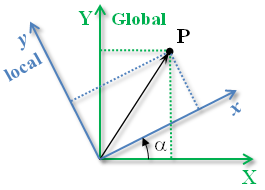A pure two-dimensional rotation of a coordinate system in relation to other coordinate system and the representation of a point in these two coordinate systems are illustrated in the figure below (remember that this is equivalent to describing a rotation between two rigid bodies). The rotation is around an axis orthogonal to this page, not shown in the figure (for a three-dimensional coordinate system the rotation would be around the $\mathbf{Z}$ axis). #
#

rotation 2D — Figure. A point in the two-dimensional space represented in two coordinate systems (Global and local), with one system rotated in relation to the other around an axis orthogonal to both coordinate systems.

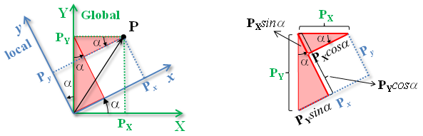
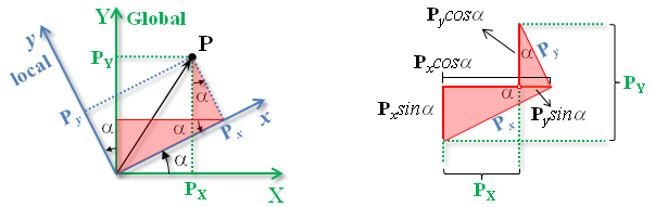
# # Consider we want to express the position of point $\mathbf{P}$ in the Global coordinate system in terms of the local coordinate system knowing only the coordinates at the local coordinate system and the angle of rotation between the two coordinate systems. # # There are different ways of deducing that, we will see three of these methods next. # ### Using trigonometry # # From figure below, the coordinates of point $\mathbf{P}$ in the Global coordinate system can be determined finding the sides of the triangles marked in red. # #
#

# # Then: # #
# # \begin{equation} # \mathbf{P_X} = \mathbf{P}_x \cos \alpha - \mathbf{P}_y \sin \alpha \\ # \\ # \mathbf{P_Y} = \mathbf{P}_x \sin \alpha + \mathbf{P}_y \cos \alpha # \end{equation} # # # The equations above can be expressed in matrix form: # #
# # \begin{equation} # \begin{bmatrix} # \mathbf{P_X} \\ # \mathbf{P_Y} # \end{bmatrix} = # \begin{bmatrix} # \cos\alpha & -\sin\alpha \\ # \sin\alpha & \hphantom{-}\cos\alpha # \end{bmatrix} \begin{bmatrix} # \mathbf{P}_x \\ # \mathbf{P}_y # \end{bmatrix} # \end{equation} # # # Or simply: # # # \begin{equation} # \mathbf{P_G} = \mathbf{R_{Gl}}\mathbf{P_l} # \end{equation} # # # Where $\mathbf{R_{Gl}}$ is the rotation matrix that rotates the coordinates from the local to the Global coordinate system: # #
# # \begin{equation} # \mathbf{R_{Gl}} = \begin{bmatrix} # \cos\alpha & -\sin\alpha \\ # \sin\alpha & \hphantom{-}\cos\alpha # \end{bmatrix} # \end{equation} # # # So, given any position at the local coordinate system, with the rotation matrix above we are able to determine the position at the Global coordinate system. Let's check that before looking at other methods to obtain this matrix. # # For instance, consider a local coordinate system rotated by $45^o$ in relation to the Global coordinate system, a point in the local coordinate system with position $\mathbf{P_l}=[1, 1]$ will have the following position at the Global coordinate system: # In[4]: α = np.pi / 4 RGl = np.array([[np.cos(α), -np.sin(α)], [np.sin(α), np.cos(α)]]) Pl = np.array([[1, 1]]).T # transpose the array for correct matrix multiplication PG = RGl @ Pl # the operator @ is used for matrix multiplication of arrays PG # And if we have the points [1,1], [0,1], [1,0] at the local coordinate system, their positions at the Global coordinate system are: # In[ ]: Pl = np.array([[1, 1], [0, 1], [1, 0]]).T # transpose array for matrix multiplication PG = RGl@Pl PG # ### Using direction cosines # # Another way to determine the rotation matrix is to use the concept of direction cosine. # # > Direction cosines are the cosines of the angles between any two vectors. 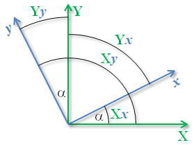# # For the present case with two coordinate systems, they are the cosines of the angles between each axis of one coordinate system and each axis of the other coordinate system. The figure below illustrates the directions angles between the two coordinate systems, expressing the local coordinate system in terms of the Global coordinate system. # #
#

direction angles 2D — *Figure. Definition of direction angles at the two-dimensional space.*

# #
# # \begin{equation} # \mathbf{R_{Gl}} = \begin{bmatrix} # \cos\mathbf{X}x & \cos\mathbf{X}y \\ # \cos\mathbf{Y}x & \cos\mathbf{Y}y # \end{bmatrix} = # \begin{bmatrix} # \cos(\alpha) & \cos(90^o+\alpha) \\ # \cos(90^o-\alpha) & \cos(\alpha) # \end{bmatrix} = # \begin{bmatrix} # \cos\alpha & -\sin\alpha \\ # \sin\alpha & \hphantom{-}\cos\alpha # \end{bmatrix} # \end{equation} # # # The same rotation matrix as obtained before. # # Note that the order of the direction cosines is because in our convention, the first row is for the $\mathbf{X}$ coordinate and the second row for the $\mathbf{Y}$ coordinate (the outputs). For the inputs, we followed the same order, first column for the $\mathbf{x}$ coordinate, second column for the $\mathbf{y}$ coordinate. 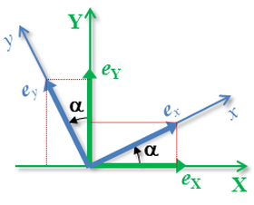# ### 3. Using a basis # # Yet another way to deduce the rotation matrix is to view the axes of the rotated coordinate system as unit vectors, versors, of a basis as illustrated in the figure below. # # > A basis is a set of linearly independent vectors that can represent every vector in a given vector space, i.e., a basis defines a coordinate system. # #

basis 2D — *Figure. Definition of the rotation matrix using a basis at the two-dimensional space.*

# # The coordinates of these two versors at the local coordinate system in terms of the Global coordinate system are: # #
# # \begin{equation} # \begin{array}{l l} # \mathbf{e}_x = \hphantom{-}\cos\alpha\:\mathbf{e_X} + \sin\alpha\:\mathbf{e_Y} \\ # \mathbf{e}_y = -\sin\alpha\:\mathbf{e_X} + \cos\alpha\:\mathbf{e_Y} # \end{array} # \end{equation} # # # Note that as unit vectors, each of the versors above should have norm (length) equals to one, which indeed is the case. # # If we express each versor above as different columns of a matrix, we obtain the rotation matrix again: # #
# # \begin{equation} # \mathbf{R_{Gl}} = \begin{bmatrix} # \cos\alpha & -\sin\alpha \\\ # \sin\alpha & \hphantom{-}\cos\alpha # \end{bmatrix} # \end{equation} # # # This means that the rotation matrix can be viewed as the basis of the rotated coordinate system defined by its versors. # # This third way to derive the rotation matrix is in fact the method most commonly used in motion analysis because the coordinates of markers (in the Global/laboratory coordinate system) are what we measure with cameras. # # Probably you are wondering how to perform the inverse operation, given a point in the Global coordinate system how to calculate its position in the local coordinate system. Let's see this now. # ### Local-to-Global and Global-to-local coordinate systems' rotations # If we want the inverse operation, to express the position of point $\mathbf{P}$ in the local coordinate system in terms of the Global coordinate system, the figure below illustrates that using trigonometry. # #
#

# # Then: # #
# # \begin{equation} # \mathbf{P}_x = \;\;\mathbf{P_X} \cos \alpha + \mathbf{P_Y} \sin \alpha # \end{equation} # # #
# # \begin{equation} # \mathbf{P}_y = -\mathbf{P_X} \sin \alpha + \mathbf{P_Y} \cos \alpha # \end{equation} # # # And in matrix form: # #
# # \begin{equation} # \begin{bmatrix} # \mathbf{P}_x \\ # \mathbf{P}_y # \end{bmatrix} = # \begin{bmatrix} # \hphantom{-}\cos\alpha & \sin\alpha \\ # -\sin\alpha & \cos\alpha # \end{bmatrix} \begin{bmatrix} # \mathbf{P_X} \\ # \mathbf{P_Y} # \end{bmatrix} # \end{equation} # # #
# # \begin{equation} # \mathbf{P_l} = \mathbf{R_{lG}}\mathbf{P_G} # \end{equation} # # # Where $\mathbf{R_{lG}}$ is the rotation matrix that rotates the coordinates from the Global to the local coordinate system (note the inverse order of the subscripts): # #
# # \begin{equation} # \mathbf{R_{lG}} = \begin{bmatrix} # \hphantom{-}\cos\alpha & \sin\alpha \\ # -\sin\alpha & \cos\alpha # \end{bmatrix} # \end{equation} # # # If we use the direction cosines to calculate the rotation matrix, because the axes didn't change, the cosines are the same, only the order changes, now $\mathbf{x, y}$ are the rows (outputs) and $\mathbf{X, Y}$ are the columns (inputs): # #
# # \begin{equation} # \mathbf{R_{lG}} = \begin{bmatrix} # \cos\mathbf{X}x & \cos\mathbf{Y}x \\ # \cos\mathbf{X}y & \cos\mathbf{Y}y # \end{bmatrix} = # \begin{bmatrix} # \cos(\alpha) & \cos(90^o-\alpha) \\ # \cos(90^o+\alpha) & \cos(\alpha) # \end{bmatrix} = # \begin{bmatrix} # \hphantom{-}\cos\alpha & \sin\alpha \\ # -\sin\alpha & \cos\alpha # \end{bmatrix} # \end{equation} # # # # And defining the versors of the axes in the Global coordinate system for a basis in terms of the local coordinate system would also produce this latter rotation matrix. # # The two sets of equations and matrices for the rotations from Global-to-local and local-to-Global coordinate systems are very similar, this is no coincidence. Each of the rotation matrices we deduced, $\mathbf{R_{Gl}}$ and $\mathbf{R_{lG}}$, perform the inverse operation in relation to the other. Each matrix is the inverse of the other. # # In other words, the relation between the two rotation matrices means it is equivalent to instead of rotating the local coordinate system by $\alpha$ in relation to the Global coordinate system, to rotate the Global coordinate system by $-\alpha$ in relation to the local coordinate system; remember that $\cos(-\alpha)=\cos(\alpha)$ and $\sin(-\alpha)=-\sin(\alpha)$. # ### The orthogonality of the rotation matrix # # **[See here for a review about matrix and its main properties](https://nbviewer.jupyter.org/github/BMClab/bmc/blob/master/notebooks/Matrix.ipynb)**. # # A nice property of the rotation matrix is that its inverse is the transpose of the matrix (because the columns/rows are mutually orthogonal and have norm equal to one). # This property can be shown with the rotation matrices we deduced: # # # \begin{equation} # \begin{array}{l l} # \mathbf{R}\:\mathbf{R^T} & = # \begin{bmatrix} # \cos\alpha & -\sin\alpha \\ # \sin\alpha & \hphantom{-}\cos\alpha # \end{bmatrix} # \begin{bmatrix} # \hphantom{-}\cos\alpha & \sin\alpha \\ # -\sin\alpha & \cos\alpha # \end{bmatrix} \\ # & = \begin{bmatrix} # \cos^2\alpha+\sin^2\alpha & \cos\alpha \sin\alpha-\sin\alpha \cos\alpha\;\; \\ # \sin\alpha \cos\alpha-\cos\alpha \sin\alpha & \sin^2\alpha+\cos^2\alpha\;\; # \end{bmatrix} \\ # & = \begin{bmatrix} # 1 & 0 \\ # 0 & 1 # \end{bmatrix} \\ # & = \mathbf{I} \\ # \mathbf{R^{-1}} = \mathbf{R^T} # \end{array} # \end{equation} # # # This means that if we have a rotation matrix, we know its inverse. # # The transpose and inverse operators in NumPy are methods of the array: # In[5]: α = np.pi/4 RGl = np.array([[np.cos(α), -np.sin(α)], [np.sin(α), np.cos(α)]]) print('Orthogonal matrix (RGl):\n', RGl) print('Transpose (RGl.T):\n', RGl.T) print('Inverse (RGl.I):\n', np.linalg.inv(RGl)) # Using the inverse and the transpose mathematical operations, the coordinates at the local coordinate system given the coordinates at the Global coordinate system and the rotation matrix can be obtained by: # #
# # \begin{equation} # \begin{array}{l l} # \mathbf{P_G} = \mathbf{R_{Gl}}\mathbf{P_l} \implies \\ # \mathbf{R_{Gl}^{-1}}\mathbf{P_G} = \mathbf{R_{Gl}^{-1}}\mathbf{R_{Gl}}\mathbf{P_l} \implies \\ # \mathbf{R_{Gl}^{-1}}\mathbf{P_G} = \mathbf{I}\:\mathbf{P_l} \implies \\ # \mathbf{P_l} = \mathbf{R_{Gl}^{-1}}\mathbf{P_G} = \mathbf{R_{Gl}^T}\mathbf{P_G} \quad \text{or} # \quad \mathbf{P_l} = \mathbf{R_{lG}}\mathbf{P_G} # \end{array} # \end{equation} # # # Where we referred the inverse of $\mathbf{R_{Gl}}\;(\:\mathbf{R_{Gl}^{-1}})$ as $\mathbf{R_{lG}}$ (note the different order of the subscripts). # # Let's show this calculation in NumPy: # In[6]: α = np.pi/4 RGl = np.array([[np.cos(α), -np.sin(α)], [np.sin(α), np.cos(α)]]) print('Rotation matrix (RGl):\n', RGl) Pl = np.array([[1, 1]]).T # transpose the array for correct matrix multiplication print('Position at the local coordinate system (Pl):\n', Pl) PG = RGl@Pl print('Position at the Global coordinate system (PG=RGl*Pl):\n', PG) Pl = RGl.T@PG print('Position at the local coordinate system using the inverse of RGl (Pl=RlG*PG):\n', Pl) # ### 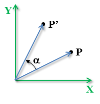Rotation of a Vector # # Another use of the rotation matrix is 'to rotate a vector by a given angle around an axis of the coordinate system as shown in the figure below. # #
#

rotation 2D of a vector — *Figure. Rotation of a position vector $\mathbf{P}$ by an angle $\alpha$ in the two-dimensional space.*

# # We will not prove that we use the same rotation matrix, but think that in this case the vector position rotates by the same angle instead of the coordinate system. The new coordinates of the vector position $\mathbf{P'}$ rotated by an angle $\alpha$ is simply the rotation matrix (for the angle $\alpha$) multiplied by the coordinates of the vector position $\mathbf{P}$: # # # \begin{equation} # \mathbf{P'} = \mathbf{R}_\alpha\mathbf{P} # \end{equation} # # # Consider for example that $\mathbf{P}=[2,1]$ and $\alpha=30^o$; the coordinates of $\mathbf{P'}$ are: # In[7]: α = np.pi/6 R = np.array([[np.cos(α), -np.sin(α)], [np.sin(α), np.cos(α)]]) P = np.array([[2, 1]]).T Pl = R@P print("P':\n", Pl) # **In summary, some of the properties of the rotation matrix are:** # 1. The columns of the rotation matrix form a basis of (independent) unit vectors (versors) and the rows are also independent versors since the transpose of the rotation matrix is another rotation matrix. # 2. The rotation matrix is orthogonal. There is no linear combination of one of the lines or columns of the matrix that would lead to the other row or column, i.e., the lines and columns of the rotation matrix are independent, orthogonal, to each other (this is property 1 rewritten). Because each row and column have norm equal to one, this matrix is also sometimes said to be orthonormal. # 3. The determinant of the rotation matrix is equal to one (or equal to -1 if a left-hand coordinate system was used, but you should rarely use that). For instance, the determinant of the rotation matrix we deduced is $\cos\alpha \cos\alpha - \sin\alpha(-\sin\alpha)=1$. # 4. The inverse of the rotation matrix is equals to its transpose. # # **On the different meanings of the rotation matrix:** # - It represents the coordinate transformation between the coordinates of a point expressed in two different coordinate systems. # - It describes the rotation between two coordinate systems. The columns are the direction cosines (versors) of the axes of the rotated coordinate system in relation to the other coordinate system and the rows are also direction cosines (versors) for the inverse rotation. # - It is an operator for the calculation of the rotation of a vector in a coordinate system. # - Rotation matrices provide a means of numerically representing rotations without appealing to angular specification. # # **Which matrix to use, from local to Global or Global to local?** # - A typical use of the transformation is in movement analysis, where there are the fixed Global (laboratory) coordinate system and the local (moving, e.g. anatomical) coordinate system attached to each body segment. Because the movement of the body segment is measured in the Global coordinate system, using cameras for example, and we want to reconstruct the coordinates of the markers at the anatomical coordinate system, we want the transformation leading from the Global coordinate system to the local coordinate system. # - Of course, if you have one matrix, it is simple to get the other; you just have to pay attention to use the right one. 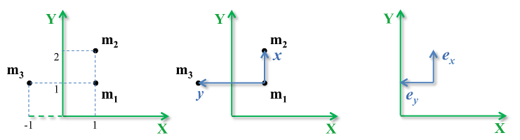# ### Calculation of rotation matrix using a basis # # A typical scenario in motion analysis is to calculate the rotation matrix using the position of markers placed on the moving rigid body. With the markers' positions, we create a local basis, which by definition is the rotation matrix for the rigid body with respect to the Global (laboratory) coordinate system. To define a coordinate system using a basís, we also will need to define an origin. # # Let's see how to calculate a basis given the markers' positions. # Consider the markers at $m1=[1,1]$, $m2=[1,2]$ and $m3=[-1,1]$ measured in the Global coordinate system as illustrated in the figure below: #
#

translation and rotation 2D — *Figure. Three points in the two-dimensional space, two possible vectors given these points, and the corresponding basis.*

# # A possible local coordinate system with origin at the position of m1 is also illustrated in the figure above. Intentionally, the three markers were chosen to form orthogonal vectors. # The translation vector between the two coordinate system is: # # # $$\mathbf{L_{Gl}} = m_1 - [0,0] = [1,1]$$ # # # The vectors expressing the axes of the local coordinate system are: # # # $$ \hat{\mathbf{x}} = m_2 - m_1 = [1,2] - [1,1] = [0,1] $$ # # $$ \hat{\mathbf{y}} = m_3 - m_1 = [-1,1] - [1,1] = [-2,0] $$ # # # Note that these two vectors do not form a basis yet because they are not unit vectors (in fact, only *y* is not a unit vector). Let's normalize these vectors: # # # $$ \begin{array}{} # \hat{\mathbf{e_x}} = \frac{x}{||x||} = \frac{[0,1]}{\sqrt{0^2+1^2}} = [0,1] \\ # \\ # \hat{\mathbf{e_y}} = \frac{y}{||y||} = \frac{[-2,0]}{\sqrt{2^2+0^2}} = [-1,0] # \end{array} $$ # # # Beware that the versors above are not exactly the same as the ones shown in the right plot of the last figure, the versors above if plotted will start at the origin of the coordinate system, not at [1,1] as shown in the figure. # # Since the markers $m1$, $m2$ and $m3$ were carefully chosen, the versors $\hat{\mathbf{e_x}}$ and $\hat{\mathbf{e_y}}$ are orthogonal. # # We could have done this calculation in NumPy (we will need to do that when dealing with real data later): # In[8]: m1 = np.array([1.,1.]) # marker 1 m2 = np.array([1.,2.]) # marker 2 m3 = np.array([-1.,1.]) # marker 3 x = m2 - m1 # vector x y = m3 - m1 # vector y vx = x/np.linalg.norm(x) # versor x vy = y/np.linalg.norm(y) # verson y print("x =", x, ", y =", y, "\nex=", vx, ", ey=", vy) # Now, both $\hat{\mathbf{e}_x}$ and $\hat{\mathbf{e}_y}$ are unit vectors (versors) and they are orthogonal, a basis can be formed with these two versors, and we can represent the rotation matrix using this basis (just place the versors of this basis as columns of the rotation matrix): # #
# # \begin{equation} # \mathbf{R_{Gl}} = \begin{bmatrix} # 0 & -1 \\ # 1 & \hphantom{-}0 # \end{bmatrix} # \end{equation} # # # This rotation matrix makes sense because from the figure above we see that the local coordinate system we defined is rotated by 90$^o$ in relation to the Global coordinate system and if we use the general form for the rotation matrix: # #
# # \begin{equation} # \mathbf{R} = \begin{bmatrix} # \cos\alpha & -\sin\alpha \\ # \sin\alpha & \hphantom{-}\cos\alpha # \end{bmatrix} = # \begin{bmatrix} # \cos90^o & -\sin90^o \\ # \sin90^o & \hphantom{-}\cos90^o # \end{bmatrix} = # \begin{bmatrix} # 0 & -1 \\ # 1 & \hphantom{-}0 # \end{bmatrix} # \end{equation} # # # So, the position of any point in the local coordinate system can be represented in the Global coordinate system by: # #
# # \begin{equation} # \begin{array}{l l} # \mathbf{P_G} =& \mathbf{L_{Gl}} + \mathbf{R_{Gl}}\mathbf{P_l} \\ # \\ # \mathbf{P_G} =& \begin{bmatrix} 1 \\ 1 \end{bmatrix} + \begin{bmatrix} 0 & -1 \\ 1 & \hphantom{-}0 \end{bmatrix} \mathbf{P_l} # \end{array} # \end{equation} # # # For example, the point $\mathbf{P_l}=[1,1]$ has the following position at the Global coordinate system: # In[9]: LGl = np.array([[1, 1]]).T print('Translation vector:\n', LGl) RGl = np.array([[0, -1], [1, 0]]) print('Rotation matrix:\n', RGl) Pl = np.array([[1, 1]]).T print('Position at the local coordinate system:\n', Pl) PG = LGl + RGl@Pl print('Position at the Global coordinate system, PG = LGl + RGl*Pl:\n', PG) # ### Determination of the unknown angle of rotation # # If we didn't know the angle of rotation between the two coordinate systems, which is the typical situation in motion analysis, we simply would equate one of the terms of the two-dimensional rotation matrix in its algebraic form to its correspondent value in the numerical rotation matrix we calculated. # #
# # \begin{equation} # \mathbf{R} = \begin{bmatrix} # \cos\alpha & -\sin\alpha \\ # \sin\alpha & \hphantom{-}\cos\alpha # \end{bmatrix} # \end{equation} # # # So the angle $\alpha$ can be found by: # #
# # \begin{equation} # \alpha = \arctan\left(\frac{R[1,0]}{R[0,0]}\right) # \end{equation} # # For instance, taking the first term of the rotation matrices above: $\cos\alpha = 0$ implies that $\alpha$ is 90$^o$ or 270$^o$, but combining with another matrix term, $\sin\alpha = 1$, implies that $\alpha=90^o$. We can solve this problem in one step using the tangent $(\sin\alpha/\cos\alpha)$ function with two terms of the rotation matrix and calculating the angle with the `arctan2(y, x)` function: # In[10]: RGl = np.array([[0, -1], [1, 0]]) ang = np.arctan2(RGl[1, 0], RGl[0, 0])*180/np.pi print('The angle is:', ang) # And this procedure would be repeated for each segment and for each instant of the analyzed movement to find the rotation of each segment. # ### Joint angle as a sequence of rotations of adjacent segments # # In the notebook about [two-dimensional angular kinematics](https://nbviewer.jupyter.org/github/BMClab/bmc/blob/master/notebooks/KinematicsAngular2D.ipynb), we calculated segment and joint angles using simple trigonometric relations. We can also calculate these two-dimensional angles using what we learned here about the rotation matrix. # # The segment angle will be given by the matrix representing the rotation from the laboratory coordinate system (G) to a coordinate system attached to the segment and the joint angle will be given by the matrix representing the rotation from one segment coordinate system (l1) to the other segment coordinate system (l2). # # So, we have to compute two basis now, one for each segment and the joint angle will be given by the product between the two rotation matrices obtained from both basis. # The description of a point P in the global basis given the description of this point in the l1 basis is: # #
# # \begin{equation} # \begin{bmatrix} # x_p\\ # y_p # \end{bmatrix} =R_{Gl1} # \begin{bmatrix} # x_{p_1}\\ # y_{p_1} # \end{bmatrix} # \end{equation} # # The description of the same point P in the global basis given the description of this point in the l2 basis is: # #
# # \begin{equation} # \begin{bmatrix} # x_p\\ # y_p # \end{bmatrix} =R_{Gl_2} # \begin{bmatrix} # x_{p_2}\\ # y_{p_2} # \end{bmatrix} # \end{equation} # # So, to find the description of this point P in the l1 basis given the description of this point in the l2 basis is: # #
# # \begin{equation} # R_{Gl_1} # \begin{bmatrix} # x_{p_1}\\ # y_{p_1} # \end{bmatrix} = # R_{Gl_2} # \begin{bmatrix} # x_{p_2}\\ # y_{p_2} # \end{bmatrix} # \rightarrow \begin{bmatrix} # x_{p_1}\\ # y_{p_1} # \end{bmatrix} = # \underbrace{R_{Gl_1}^{-1}R_{Gl_2}}_{R_{l_1l_2}} # \begin{bmatrix} # x_{p_2}\\ # y_{p_2} # \end{bmatrix} # \end{equation} # # # The rotation matrix from $l_2$ to $l_1$ is: # #
# # \begin{equation} # R_{l_1l_2} = R_{Gl_1}^{-1}R_{Gl_2} = R_{Gl_1}^{T}R_{Gl_2} # \end{equation} # # The rotation matrices of both basis are: # #
# # \begin{equation} # R_{Gl_1} = \begin{bmatrix} # \cos(\theta_1) &-\sin(\theta_1)\\ # \sin(\theta_1) &\hphantom{-}\cos(\theta_1) # \end{bmatrix}, \, # R_{Gl_2} = \begin{bmatrix} # \cos(\theta_2) &-\sin(\theta_2)\\ # \sin(\theta_2) &\hphantom{-}\cos(\theta_2) # \end{bmatrix} # \end{equation} # # # So, the rotation matrix from $l_2$ to $l_1$ is: # #
# # \begin{align} # R_{l_1l_2} =& \begin{bmatrix} # \cos(\theta_1) &\sin(\theta_1)\\ # -\sin(\theta_1) &\cos(\theta_1) # \end{bmatrix}.\begin{bmatrix} # \cos(\theta_2) &-\sin(\theta_2)\\ # \sin(\theta_2) &\hphantom{-}\cos(\theta_2) # \end{bmatrix} =\\ # =&\begin{bmatrix} # \cos(\theta_1)\cos(\theta_2)+\sin(\theta_1)\sin(\theta_2) &\cos(\theta_2)\sin(\theta_1)-\cos(\theta_1)\sin(\theta_2)\\ # \cos(\theta_1)\sin(\theta_2)-\cos(\theta_2)\sin(\theta_1)&\cos(\theta_1)\cos(\theta_2)+\sin(\theta_1)\sin(\theta_2) # \end{bmatrix}=\\ # =&\begin{bmatrix} \cos(\theta_2-\theta_1) &-\sin(\theta_2-\theta_1)\\ # \sin(\theta_2-\theta_1) &\hphantom{-}\cos(\theta_2-\theta_1) # \end{bmatrix} # \end{align} # # # The angle $\theta_{l_1l_2} = \theta_2-\theta_1$ is the angle between the two reference frames. So to find the $\theta_{l_1l_2}$ is: # #
# # \begin{align} # \theta_{l_1l_2} = \arctan\left(\frac{R_{l_1l_2}[1,0]}{R_{l_1l_2}[0,0]}\right) # \end{align} # # Below is an example: To define a two-dimensional basis, we need to calculate vectors perpendicular to each of these lines. Here is a way of doing that. First, let's find three non-collinear points for each basis: # In[11]: x1, y1, x2, y2 = 0, 0, 1, 1 # points at segment 1 x3, y3, x4, y4 = 1.1, 1, 2.1, 0 # points at segment 2 #The slope of the perpendicular line is minus the inverse of the slope of the line xl1 = x1 - (y2-y1); yl1 = y1 + (x2-x1) # point at the perpendicular line 1 xl2 = x4 - (y3-y4); yl2 = y4 + (x3-x4) # point at the perpendicular line 2 # With these three points, we can create a basis and the corresponding rotation matrix: # In[12]: b1x = np.array([x2-x1, y2-y1]) b1x = b1x/np.linalg.norm(b1x) # versor x of basis 1 b1y = np.array([xl1-x1, yl1-y1]) b1y = b1y/np.linalg.norm(b1y) # versor y of basis 1 b2x = np.array([x3-x4, y3-y4]) b2x = b2x/np.linalg.norm(b2x) # versor x of basis 2 b2y = np.array([xl2-x4, yl2-y4]) b2y = b2y/np.linalg.norm(b2y) # versor y of basis 2 RGl1 = np.array([b1x, b1y]).T # rotation matrix from segment 1 to the laboratory RGl2 = np.array([b2x, b2y]).T # rotation matrix from segment 2 to the laboratory print('rotation matrix from segment 1 to global:\n', RGl1) print('rotation matrix from segment 2 to global:\n', RGl2) # Now, the segment and joint angles are simply matrix operations: # In[13]: print('Rotation matrix for segment 1:\n', RGl1) print('\nRotation angle of segment 1:', np.arctan2(RGl1[1,0], RGl1[0,0])*180/np.pi) print('\nRotation matrix for segment 2:\n', RGl2) print('\nRotation angle of segment 2:', np.arctan2(RGl1[1,0], RGl2[0,0])*180/np.pi) Rl1l2 = RGl1.T@RGl2 # Rl1l2 = Rl1G*RGl2 print('\nJoint rotation matrix (Rl1l2 = Rl1G*RGl2):\n', Rl1l2) print('\nJoint angle:', np.arctan2(Rl1l2[1,0], Rl1l2[0,0])*180/np.pi) # Same result as obtained in [Angular kinematics in a plane (2D)](https://nbviewer.jupyter.org/github/BMClab/bmc/blob/master/notebooks/KinematicsAngular2D.ipynb). # ### Kinematic chain in a plain (2D) # # The fact that we simply multiplied the rotation matrices to calculate the rotation matrix of one segment in relation to the other is powerful and can be generalized for any number of segments: given a serial kinematic chain with links 1, 2, ..., n and 0 is the base/laboratory, the rotation matrix between the base and last link is: $\mathbf{R_{n,n-1}R_{n-1,n-2} \dots R_{2,1}R_{1,0}}$, where each matrix in this product (calculated from right to left) is the rotation of one link with respect to the next one. # # For instance, consider a kinematic chain with two links, the link 1 is rotated by $\alpha_1$ with respect to the base (0) and the link 2 is rotated by $\alpha_2$ with respect to the link 1. # Using Sympy, the rotation matrices for link 2 w.r.t. link 1 $(R_{12})$ and for link 1 w.r.t. base 0 $(R_{01})$ are: # In[14]: from IPython.display import display, Math from sympy import sin, cos, Matrix, simplify, latex, symbols from sympy.interactive import printing printing.init_printing() # In[15]: a1, a2 = symbols('alpha1 alpha2') R12 = Matrix([[cos(a2), -sin(a2)], [sin(a2), cos(a2)]]) display(Math(r'\mathbf{R_{12}}=' + latex(R12))) R01 = Matrix([[cos(a1), -sin(a1)], [sin(a1), cos(a1)]]) display(Math(r'\mathbf{R_{01}}=' + latex(R01))) # The rotation matrix of link 2 w.r.t. the base $(R_{02})$ is given simply by $R_{01}*R_{12}$: # In[16]: R02 = R01*R12 display(Math(r'\mathbf{R_{02}}=' + latex(R02))) # Which simplifies to: # In[17]: display(Math(r'\mathbf{R_{02}}=' + latex(simplify(R02)))) # As expected. # # The typical use of all these concepts is in the three-dimensional motion analysis where we will have to deal with angles in different planes, which needs a special manipulation as we will see next. 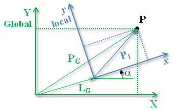# ## Translation and rotation # # Consider now the case where the local coordinate system is translated and rotated in relation to the Global coordinate system and a point is described in both coordinate systems as illustrated in the figure below (once again, remember that this is equivalent to describing a translation and a rotation between two rigid bodies). #
#

# # The position of point $\mathbf{P}$ originally described in the local coordinate system, but now described in the Global coordinate system in vector form is: # #
# # \begin{equation} # \mathbf{P_G} = \mathbf{L_G} + \mathbf{R_{Gl}}\mathbf{P_l} # \end{equation} # # # And in matrix form: # #
# # \begin{equation} # \begin{bmatrix} # \mathbf{P_X} \\ # \mathbf{P_Y} # \end{bmatrix} = # \begin{bmatrix} \mathbf{L_{X}} \\\ \mathbf{L_{Y}} \end{bmatrix} + # \begin{bmatrix} # \cos\alpha & -\sin\alpha \\ # \sin\alpha & \hphantom{-}\cos\alpha # \end{bmatrix} \begin{bmatrix} # \mathbf{P}_x \\ # \mathbf{P}_y # \end{bmatrix} # \end{equation} # # # This means that we first *disrotate* the local coordinate system and then correct for the translation between the two coordinate systems. Note that we can't invert this order: the point position is expressed in the local coordinate system and we can't add this vector to another vector expressed in the Global coordinate system, first we have to convert the vectors to the same coordinate system. # # If now we want to find the position of a point at the local coordinate system given its position in the Global coordinate system, the rotation matrix and the translation vector, we have to invert the expression above: # #
# # \begin{equation} # \begin{array}{l l} # \mathbf{P_G} = \mathbf{L_G} + \mathbf{R_{Gl}}\mathbf{P_l} \implies \\ # \mathbf{R_{Gl}^{-1}}(\mathbf{P_G} - \mathbf{L_G}) = \mathbf{R_{Gl}^{-1}}\mathbf{R_{Gl}}\mathbf{P_l} \implies \\ # \mathbf{P_l} = \mathbf{R_{Gl}^{-1}}\left(\mathbf{P_G}-\mathbf{L_G}\right) = \mathbf{R_{Gl}^T}\left(\mathbf{P_G}-\mathbf{L_G}\right) \quad \text{or} \quad \mathbf{P_l} = \mathbf{R_{lG}}\left(\mathbf{P_G}-\mathbf{L_G}\right) # \end{array} # \end{equation} # # # The expression above indicates that to perform the inverse operation, to go from the Global to the local coordinate system, we first translate and then rotate the coordinate system. # ### Transformation matrix # # It is possible to combine the translation and rotation operations in only one matrix, called the transformation matrix (also referred as homogeneous transformation matrix): # #
# # \begin{equation} # \begin{bmatrix} # \mathbf{P_X} \\ # \mathbf{P_Y} \\ # 1 # \end{bmatrix} = # \begin{bmatrix} # \cos\alpha & -\sin\alpha & \mathbf{L_{X}} \\ # \sin\alpha & \hphantom{-}\cos\alpha & \mathbf{L_{Y}} \\ # 0 & 0 & 1 # \end{bmatrix} \begin{bmatrix} # \mathbf{P}_x \\ # \mathbf{P}_y \\ # 1 # \end{bmatrix} # \end{equation} # # # Or simply: # #
# # \begin{equation} # \mathbf{P_G} = \mathbf{T_{Gl}}\mathbf{P_l} # \end{equation} # # # The inverse operation, to express the position at the local coordinate system in terms of the Global coordinate system, is: # #
# # \begin{equation} # \mathbf{P_l} = \mathbf{T_{Gl}^{-1}}\mathbf{P_G} # \end{equation} # # # However, because $\mathbf{T_{Gl}}$ is not orthonormal, which means its inverse is not its transpose. Its inverse in matrix form is given by: # #
# # \begin{equation} # \begin{bmatrix} # \mathbf{P}_x \\ # \mathbf{P}_y \\ # 1 # \end{bmatrix} = # \underbrace{\begin{bmatrix} # \mathbf{R^{-1}_{Gl}} & \cdot & - \mathbf{R^{-1}_{Gl}}\mathbf{L_{G}} \\ # \cdot & \cdot & \cdot \\ # 0 & 0 & 1 # \end{bmatrix}}_{ \mathbf{T_{Gl}^{-1}}} \begin{bmatrix} # \mathbf{P_X} \\ # \mathbf{P_Y} \\ # 1 # \end{bmatrix} # \end{equation} # # ## Further reading # # - Read pages 751-758 of the 16th chapter of the [Ruina and Rudra's book](http://ruina.tam.cornell.edu/Book/index.html) about rotation matrix # - Read section 2.8 of Rade's book about using the concept of rotation matrix applied to kinematic chains # - [Rotation matrix](https://en.wikipedia.org/wiki/Rotation_matrix) - Wikipedia # ## Video lectures on the Internet # # - [Linear transformation examples: Rotations in R2](https://www.khanacademy.org/math/linear-algebra/matrix-transformations/lin-trans-examples/v/linear-transformation-examples-rotations-in-r2) - Khan Academy # - [Linear transformations and matrices | Chapter 3, Essence of linear algebra](https://youtu.be/kYB8IZa5AuE) - 3Blue1Brown # - [Linear Transformations and Their Matrices](https://youtu.be/Ts3o2I8_Mxc) - MIT OpenCourseWare # - [Rotation Matrices](https://youtu.be/4srS0s1d9Yw) # ## Problems # # 1. A local coordinate system is rotated 30$^o$ clockwise in relation to the Global reference system. # A. Determine the matrices for rotating one coordinate system to another (two-dimensional). # B. What are the coordinates of the point [1, 1] (local coordinate system) at the global coordinate system? # C. And if this point is at the Global coordinate system and we want the coordinates at the local coordinate system? # D. Consider that the local coordinate system, besides the rotation is also translated by [2, 2]. What are the matrices for rotation, translation, and transformation from one coordinate system to another (two-dimensional)? # E. Repeat B and C considering this translation. # # 2. Consider a local coordinate system U rotated 45$^o$ clockwise in relation to the Global reference system and another local coordinate system V rotated 45$^o$ clockwise in relation to the local reference system U. # A. Determine the rotation matrices of all possible transformations between the coordinate systems. # B. For the point [1, 1] in the coordinate system U, what are its coordinates in coordinate system V and in the Global coordinate system? # # 3. Using the rotation matrix, deduce the new coordinates of a square figure with coordinates [0, 0], [1, 0], [1, 1], and [0, 1] when rotated by 0$^o$, 45$^o$, 90$^o$, 135$^o$, and 180$^o$ (always clockwise). # # 4. Solve the problem 2 of [Angular kinematics in a plane (2D)](https://nbviewer.jupyter.org/github/BMClab/bmc/blob/master/notebooks/KinematicsAngular2D.ipynb) but now using the concept of two-dimensional transformations. # # 5. Write a Python code to solve the problem in [https://leetcode.com/problems/rotate-image/](https://leetcode.com/problems/rotate-image/). # # 6. Rotate a triangle placed at A(0,0), B(1,1) and C(5,2) by an angle $45^o$ with respect to origin. From https://studyresearch.in/2019/12/14/numerical-example-of-rotation-in-2d-transformation/. # # 7. Rotate a triangle placed at A(0,0), B(1,1) and C(5,2) by an angle $45^o$ with respect to point P(-1,-1). From https://studyresearch.in/2019/12/14/numerical-example-of-rotation-in-2d-transformation/. # # ## References # # - Rade D (2017) [Cinemática e Dinâmica para Engenharia](https://www.grupogen.com.br/e-book-cinematica-e-dinamica-para-engenharia). Grupo GEN. # - Robertson G, Caldwell G, Hamill J, Kamen G (2013) [Research Methods in Biomechanics](http://books.google.com.br/books?id=gRn8AAAAQBAJ). 2nd Edition. Human Kinetics. # - Ruina A, Rudra P (2013) [Introduction to Statics and Dynamics](http://ruina.tam.cornell.edu/Book/index.html). Oxford University Press. # - Winter DA (2009) [Biomechanics and motor control of human movement](http://books.google.com.br/books?id=_bFHL08IWfwC). 4 ed. Hoboken, EUA: Wiley. # - Zatsiorsky VM (1997) [Kinematics of Human Motion](http://books.google.com.br/books/about/Kinematics_of_Human_Motion.html?id=Pql_xXdbrMcC&redir_esc=y). Champaign, Human Kinetics.

Contents