#!/usr/bin/env python
# coding: utf-8
# # 09 - Introduction to Neural Networks
#
# by [Fabio A. González](http://dis.unal.edu.co/~fgonza/), Universidad Nacional de Colombia
#
# version 1.0, June 2018
#
# ## Part of the class [Applied Deep Learning](https://github.com/albahnsen/AppliedDeepLearningClass)
#
#
# This notebook is licensed under a [Creative Commons Attribution-ShareAlike 3.0 Unported License](http://creativecommons.org/licenses/by-sa/3.0/deed.en_US).
#
#
# To run this notebook you need to download Pybrain (https://github.com/pybrain/pybrain) and copy the `pybrain` folder to the same folder where this notebook is.
#
#
# In[2]:
import pybrain
import numpy as np
import pandas as pd
from matplotlib import pyplot as plt
get_ipython().run_line_magic('matplotlib', 'inline')
# ## Artificial Neuron
#
#  #
# $$o_j^{(n)} = \varphi\left(\sum_{i\; in\; layer (n-1)}w_{ij}o_i^{(n-1)} \right)$$
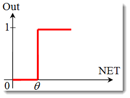
# ## Step activation function
#
#
# $$o_j^{(n)} = \varphi\left(\sum_{i\; in\; layer (n-1)}w_{ij}o_i^{(n-1)} \right)$$
# ## Step activation function
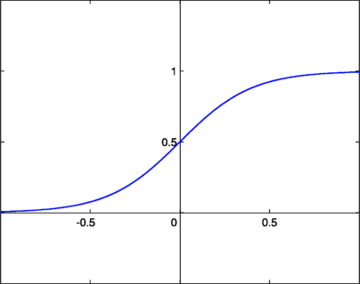
#  # ## Logistic activation function
#
# $$\varphi(x) = \frac{1}{1 - e^{-(x-b)}}$$
#
#
# ## Logistic activation function
#
# $$\varphi(x) = \frac{1}{1 - e^{-(x-b)}}$$
#
#  # ### Question: How to program an artificial neuron to calculate the *and* function?
#
# ### Question: How to program an artificial neuron to calculate the *and* function?
#
#
#
# | $X$ |
# $Y$ |
# $X$ and $Y$ |
#
#
# | 0 |
# 0 |
# 0 |
#
#
# | 0 |
# 1 |
# 0 |
#
#
# | 1 |
# 0 |
# 0 |
#
#
# | 1 |
# 1 |
# 1 |
#
#
# ## AND Neural Network
#
#  # In[3]:
from pybrain.tools.shortcuts import buildNetwork
net = buildNetwork(2, 1, outclass=pybrain.SigmoidLayer)
print(net.params)
# In[4]:
def print_pred2(dataset, network):
df = pd.DataFrame(dataset.data['sample'][:dataset.getLength()],columns=['X', 'Y'])
prediction = np.round(network.activateOnDataset(dataset),3)
df['output'] = pd.DataFrame(prediction)
return df
from pybrain.datasets import UnsupervisedDataSet, SupervisedDataSet
D = UnsupervisedDataSet(2) # define a dataset in pybrain
D.addSample([0,0])
D.addSample([0,1])
D.addSample([1,0])
D.addSample([1,1])
print_pred2(D, net)
# ## AND Neural Network
#
# In[5]:
net.params[:] = [ -150, -100, 100]
print_pred2(D, net)
# ### Question: How to program an artificial neuron to calculate the *xor* function?
#
# In[3]:
from pybrain.tools.shortcuts import buildNetwork
net = buildNetwork(2, 1, outclass=pybrain.SigmoidLayer)
print(net.params)
# In[4]:
def print_pred2(dataset, network):
df = pd.DataFrame(dataset.data['sample'][:dataset.getLength()],columns=['X', 'Y'])
prediction = np.round(network.activateOnDataset(dataset),3)
df['output'] = pd.DataFrame(prediction)
return df
from pybrain.datasets import UnsupervisedDataSet, SupervisedDataSet
D = UnsupervisedDataSet(2) # define a dataset in pybrain
D.addSample([0,0])
D.addSample([0,1])
D.addSample([1,0])
D.addSample([1,1])
print_pred2(D, net)
# ## AND Neural Network
#
# In[5]:
net.params[:] = [ -150, -100, 100]
print_pred2(D, net)
# ### Question: How to program an artificial neuron to calculate the *xor* function?
#
#
#
# | $X$ |
# $Y$ |
# $X$ xor $Y$ |
#
#
# | 0 |
# 0 |
# 0 |
#
#
# | 0 |
# 1 |
# 1 |
#
#
# | 1 |
# 0 |
# 1 |
#
#
# | 1 |
# 1 |
# 0 |
#
#
# ## Plotting the NN Output
# In[6]:
def plot_nn_prediction(N):
# a function to plot the binary output of a network on the [0,1]x[0,1] space
x_list = np.arange(0.0,1.0,0.025)
y_list = np.arange(1.0,0.0,-0.025)
z = [0.0 if N.activate([x,y])[0] <0.5 else 1.0 for y in y_list for x in x_list]
z = np.array(z)
grid = z.reshape((len(x_list), len(y_list)))
plt.imshow(grid, extent=(x_list.min(), x_list.max(), y_list.min(), y_list.max()),cmap=plt.get_cmap('Greys_r'))
plt.show()
# ## Plotting the NN Output
# In[7]:
net.params[:] = [-20, -50, 50]
plot_nn_prediction(net)
#
#
# ## Answer: It is impossible with only one neuron!
#
#
#
# ## We need to use more than one neuron....
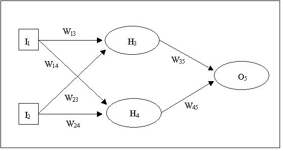
# ## Multilayer Neural Network
#  # ## Learning an XOR NN
# In[8]:
Dtrain = SupervisedDataSet(2,1) # define a dataset in pybrain
Dtrain.addSample([0,0],[0])
Dtrain.addSample([0,1],[1])
Dtrain.addSample([1,0],[1])
Dtrain.addSample([1,1],[0])
from pybrain.supervised.trainers import BackpropTrainer
net = buildNetwork(2, 2, 1, hiddenclass=pybrain.SigmoidLayer, outclass=pybrain.SigmoidLayer)
T = BackpropTrainer(net, learningrate=0.1, momentum=0.9)
T.trainOnDataset(Dtrain, 1000)
print_pred2(D, net)
# ## XOR NN Output Plot
# In[9]:
plot_nn_prediction(net)
# ## The Little Red Riding Hood Neural Network
#
#
# ## Learning an XOR NN
# In[8]:
Dtrain = SupervisedDataSet(2,1) # define a dataset in pybrain
Dtrain.addSample([0,0],[0])
Dtrain.addSample([0,1],[1])
Dtrain.addSample([1,0],[1])
Dtrain.addSample([1,1],[0])
from pybrain.supervised.trainers import BackpropTrainer
net = buildNetwork(2, 2, 1, hiddenclass=pybrain.SigmoidLayer, outclass=pybrain.SigmoidLayer)
T = BackpropTrainer(net, learningrate=0.1, momentum=0.9)
T.trainOnDataset(Dtrain, 1000)
print_pred2(D, net)
# ## XOR NN Output Plot
# In[9]:
plot_nn_prediction(net)
# ## The Little Red Riding Hood Neural Network
#
#  # ## LRRH Network Architecture
#
#
# ## LRRH Network Architecture
#
#  # ## Training
#
# In[10]:
from pybrain.tools.validation import Validator
validator = Validator()
Dlrrh = SupervisedDataSet(4,4)
Dlrrh.addSample([1,1,0,0],[1,0,0,0])
Dlrrh.addSample([0,1,1,0],[0,0,1,1])
Dlrrh.addSample([0,0,0,1],[0,1,1,0])
df = pd.DataFrame(Dlrrh['input'],columns=['Big Ears', 'Big Teeth', 'Handsome', 'Wrinkled'])
print (df.join(pd.DataFrame(Dlrrh['target'],columns=['Scream', 'Hug', 'Food', 'Kiss'])))
net = buildNetwork(4, 3, 4, hiddenclass=pybrain.SigmoidLayer, outclass=pybrain.SigmoidLayer)
# ## Backpropagation
# In[11]:
T = BackpropTrainer(net, learningrate=0.01, momentum=0.99)
scores = []
for i in range(1000):
T.trainOnDataset(Dlrrh, 1)
prediction = net.activateOnDataset(Dlrrh)
scores.append(validator.MSE(prediction, Dlrrh.getField('target')))
plt.ylabel('Mean Square Error')
plt.xlabel('Iteration')
plt.plot(scores)
# ## Learning as optimization
#
# General optimization problem:
#
# $$\min_{f\in H}L(f,D)$$
#
# with $H$: hypothesis space, $D$:training data, $L$:loss/error
# ## Example, least squares linear regression:
# $$\min_{f\in H}L(f,D)$$
# * Hypothesis space:
# $f(x)=w^{T}x$
# * Data: $D = \{(x_1, t_1), \dots , (x_n, t_n)\}$
# * Least squares loss:
# $$L(f, D)=-\sum_{t_i \in D}(t_{i} - f(x_i))^2$$
# ## Example, logistic regression:
# $$\min_{f\in H}L(f,D)$$
# * Hypothesis space:
# $f(x)=P(C_{+}|x)=\sigma(w^{T}x)$
# * Data: $D = \{(x_1, t_1), \dots , (x_n, t_n)\}$
# * Cross-entropy error:
# $$E(f,D)=-\ln p(D|f)=-\sum_{t_i \in D}(t_{n}\ln y_{n}+(1-t_{n})\ln(1-y_{n}))$$
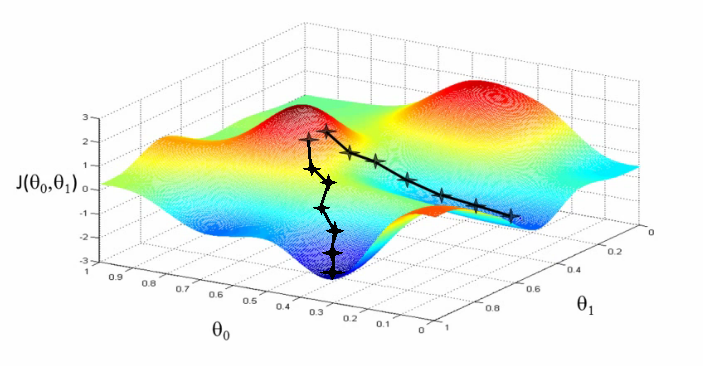
# ## Gradient descent
#
#
# ## Training
#
# In[10]:
from pybrain.tools.validation import Validator
validator = Validator()
Dlrrh = SupervisedDataSet(4,4)
Dlrrh.addSample([1,1,0,0],[1,0,0,0])
Dlrrh.addSample([0,1,1,0],[0,0,1,1])
Dlrrh.addSample([0,0,0,1],[0,1,1,0])
df = pd.DataFrame(Dlrrh['input'],columns=['Big Ears', 'Big Teeth', 'Handsome', 'Wrinkled'])
print (df.join(pd.DataFrame(Dlrrh['target'],columns=['Scream', 'Hug', 'Food', 'Kiss'])))
net = buildNetwork(4, 3, 4, hiddenclass=pybrain.SigmoidLayer, outclass=pybrain.SigmoidLayer)
# ## Backpropagation
# In[11]:
T = BackpropTrainer(net, learningrate=0.01, momentum=0.99)
scores = []
for i in range(1000):
T.trainOnDataset(Dlrrh, 1)
prediction = net.activateOnDataset(Dlrrh)
scores.append(validator.MSE(prediction, Dlrrh.getField('target')))
plt.ylabel('Mean Square Error')
plt.xlabel('Iteration')
plt.plot(scores)
# ## Learning as optimization
#
# General optimization problem:
#
# $$\min_{f\in H}L(f,D)$$
#
# with $H$: hypothesis space, $D$:training data, $L$:loss/error
# ## Example, least squares linear regression:
# $$\min_{f\in H}L(f,D)$$
# * Hypothesis space:
# $f(x)=w^{T}x$
# * Data: $D = \{(x_1, t_1), \dots , (x_n, t_n)\}$
# * Least squares loss:
# $$L(f, D)=-\sum_{t_i \in D}(t_{i} - f(x_i))^2$$
# ## Example, logistic regression:
# $$\min_{f\in H}L(f,D)$$
# * Hypothesis space:
# $f(x)=P(C_{+}|x)=\sigma(w^{T}x)$
# * Data: $D = \{(x_1, t_1), \dots , (x_n, t_n)\}$
# * Cross-entropy error:
# $$E(f,D)=-\ln p(D|f)=-\sum_{t_i \in D}(t_{n}\ln y_{n}+(1-t_{n})\ln(1-y_{n}))$$
# ## Gradient descent
#
#  # ## Prediction
# In[12]:
def lrrh_input(vals):
return pd.DataFrame(vals,index=['big ears', 'big teeth', 'handsome', 'wrinkled'], columns=['input'])
def lrrh_output(vals):
return pd.DataFrame(vals,index=['scream', 'hug', 'offer food', 'kiss cheek'], columns=['output'])
# In[13]:
in_vals = [0, 0, 0, 0]
lrrh_input(in_vals)
# In[14]:
lrrh_output(net.activate(in_vals))
# ## Prediction
# In[12]:
def lrrh_input(vals):
return pd.DataFrame(vals,index=['big ears', 'big teeth', 'handsome', 'wrinkled'], columns=['input'])
def lrrh_output(vals):
return pd.DataFrame(vals,index=['scream', 'hug', 'offer food', 'kiss cheek'], columns=['output'])
# In[13]:
in_vals = [0, 0, 0, 0]
lrrh_input(in_vals)
# In[14]:
lrrh_output(net.activate(in_vals))