#!/usr/bin/env python
# coding: utf-8
# # Linear Layer
# We will be implementing a **Linear Layer** as they are a fundamental operation in DL. The objective of a linear layer is to map a fixed number of inputs to a desired output (whether it be a regression or classification task)
#
#
# ### Forward Pass
#
# A neural network architecture consists of 2 main layers: first layer (**input**) and last layer (**output**).
#
# **Node** or **neuron** is the simplest unit of the neural network. Each neuron held a numerical value that will be passed (forward direction in this case) to the next neuron by a mapping. For the sake of simplicity, we will only discuss the **linear neural network** and linear mapping in this lesson.
#
# Let's consider a simple connection between 2 layers, each has 1 neuron,
#
# 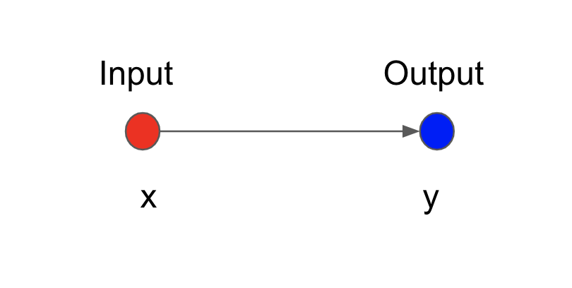 #
# We can map the input neuron $x$ to the output neuron $y$ by a linear equation,
#
# $$ y = wx + \beta $$
#
# where $w$ is called the **weight** and $\beta$ is called the **bias term**.
#
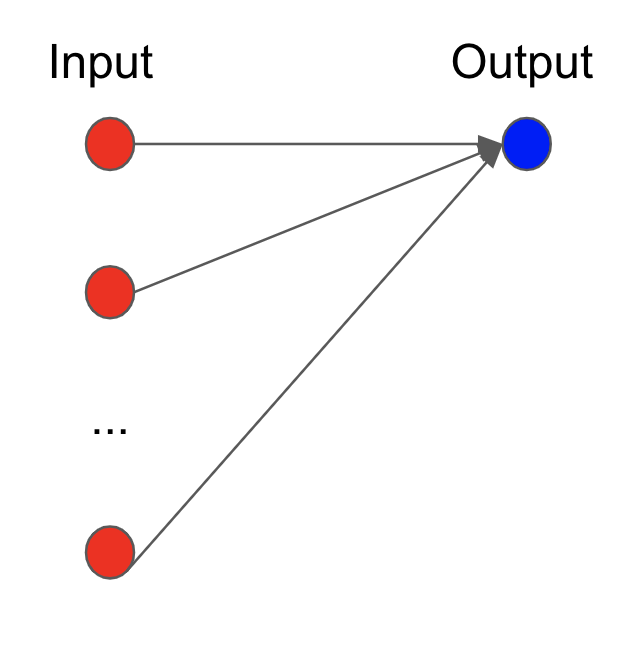
# If we have $n$ input neurons ($n>1$) then the output neuron is the linear combination,
#
#
#
# We can map the input neuron $x$ to the output neuron $y$ by a linear equation,
#
# $$ y = wx + \beta $$
#
# where $w$ is called the **weight** and $\beta$ is called the **bias term**.
#
# If we have $n$ input neurons ($n>1$) then the output neuron is the linear combination,
#
#  #
#
# $$
# \hat{y}=\beta + x_1w_1+x_2w_2+ \cdots +x_{n}w_n
# $$
#
# where $w_i$'s are weights corresponding to each map (or arrow).
#
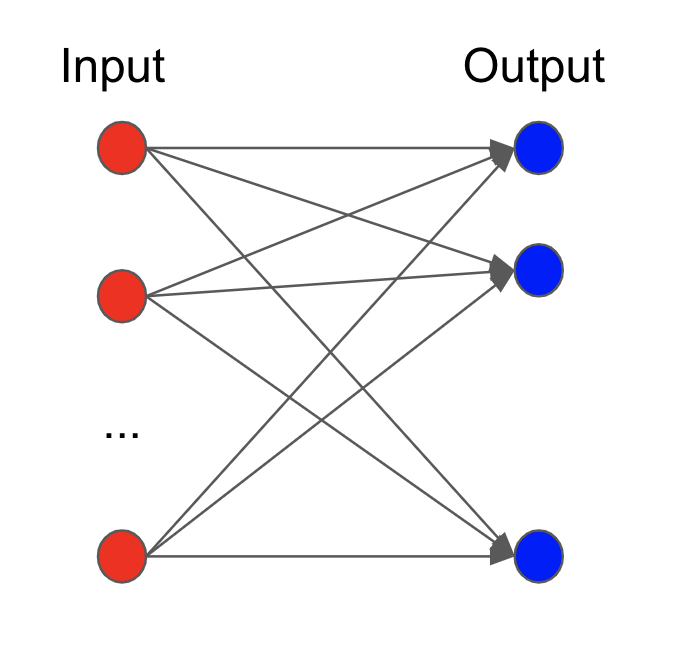
# Similarly, if there are $m$ output neurons then the ouput is the system of multi-linear equations,
#
#
#
#
# $$
# \hat{y}=\beta + x_1w_1+x_2w_2+ \cdots +x_{n}w_n
# $$
#
# where $w_i$'s are weights corresponding to each map (or arrow).
#
# Similarly, if there are $m$ output neurons then the ouput is the system of multi-linear equations,
#
#  #
#
# $$\hat{y_1}=\beta_1 + x_1 w_{1,1}+x_2 w_{1,2}+ \cdots +x_nw_{1,n} $$
#
# $$\hat{y_2}=\beta_2 + x_2 w_{2,1}+x_2 w_{2,2}+ \cdots +x_nw_{2,n} $$
# $$ \vdots $$
# $$\hat{y_m}=\beta_m + x_n w_{m,1}+x_2 w_{m,2}+ \cdots +x_nw_{m,n} $$
#
# Compactedly, it can be written in matrix form
# $$
# \hat{Y}
# = \left(\begin{array}{c} \hat{y}_{0} \\ \hat{y}_{1} \\ \vdots \\ \hat{y}_{m} \end{array}\right)
# = \left(\begin{array}{ccccc}
# \beta_1 & w_{1,1} & w_{1,2} & \cdots & w_{1,n} \\
# \beta_2 & w_{2,1} & w_{2,2} & \cdots & w_{2,n} \\
# \vdots & \vdots & \vdots & \vdots & \vdots \\
# \beta_m & w_{m,1} & w_{m,2} & \cdots & w_{m,n}
# \end{array}\right)
# \cdot \left(\begin{array}{c} x_{1} \\ x_{1} \\ \vdots \\ x_m \end{array}\right)
# = W \cdot X
# $$
#
# This logic can be extented further as we increase more layers.
#
#
#
#
# $$\hat{y_1}=\beta_1 + x_1 w_{1,1}+x_2 w_{1,2}+ \cdots +x_nw_{1,n} $$
#
# $$\hat{y_2}=\beta_2 + x_2 w_{2,1}+x_2 w_{2,2}+ \cdots +x_nw_{2,n} $$
# $$ \vdots $$
# $$\hat{y_m}=\beta_m + x_n w_{m,1}+x_2 w_{m,2}+ \cdots +x_nw_{m,n} $$
#
# Compactedly, it can be written in matrix form
# $$
# \hat{Y}
# = \left(\begin{array}{c} \hat{y}_{0} \\ \hat{y}_{1} \\ \vdots \\ \hat{y}_{m} \end{array}\right)
# = \left(\begin{array}{ccccc}
# \beta_1 & w_{1,1} & w_{1,2} & \cdots & w_{1,n} \\
# \beta_2 & w_{2,1} & w_{2,2} & \cdots & w_{2,n} \\
# \vdots & \vdots & \vdots & \vdots & \vdots \\
# \beta_m & w_{m,1} & w_{m,2} & \cdots & w_{m,n}
# \end{array}\right)
# \cdot \left(\begin{array}{c} x_{1} \\ x_{1} \\ \vdots \\ x_m \end{array}\right)
# = W \cdot X
# $$
#
# This logic can be extented further as we increase more layers.
#
# 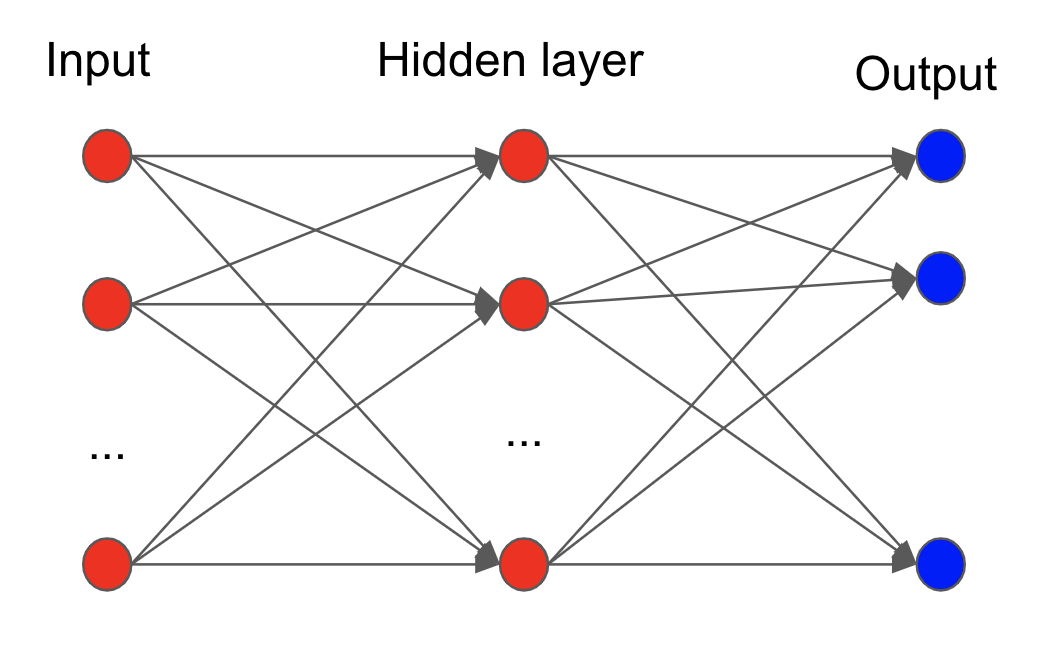 #
# The second layer (and beyond) is called the **hidden layer**. The number of hidden layer is usually decided by the complexity of the problem.
#
# **Fact:**
#
# * If the weight $w_i\neq 0$ for all $i$, then we have a **fully connected neural network.**
#
# * The number of of neuron for each layers can be different. Moreover, they tend to decrease sequentially. Ex:
# $$500 \text{ neurons} \rightarrow 100 \text{ neurons} \rightarrow 20 \text{ neurons} $$
#
# * Most of the practical neural networks are non-linear. This result is achieved by applying a non-linear function on top of the linear combination. This is called the **activation function**.
# ### Backward Pass
#
# Now that we know how to implement the forward pass, we must next solve how it is that we are going to backpropagate our linear operation.
#
# Keep in mind that backpropagation is simply the gradient of our latest forward operation (call it $o$) w.r.t. our weight parameters $w$, which, if many intermediate operations have been performed, we attain by the chain-rule
#
# $$
# \hat{y} = 1w_0+x_1w_1+x_2w_2+x_3w_3\\z = \sigma(\hat{y}) \\
# o = L(z,y)
# $$
#
# $$
# \frac{\partial o}{\partial w} = \frac{\partial o}{\partial z}*\frac{\partial z}{\partial \hat{y}}*\frac{\partial \hat{y}}{\partial w}
# $$
#
# Now, notice that during the backward pass, partial gradients can be classified in two ways:
#
# 1. An **Intermediate operation** ($\frac{\partial o}{\partial z},\frac{\partial z}{\partial \hat{y}}$) or
# 2. A **"Receiver" operation** ($\frac{\partial \hat{y}}{\partial w}$)
#
# Notice that the intermediates have to be calculated to get to our "Receiver" operation, which receives a "step" operation once its gradient has been calculated.
#
# In the above example, none of our intermediate operations introduced any new parameters to our model. However, what if they did? Look below
#
# $$
# \hat{y_1} = 1w_0+x_1w_1+x_2w_2+x_3w_3\\z = \sigma(\hat{y})\\l = z*w_4 \\o = L(l,y)
# $$
#
# $$
# \frac{\partial o}{\partial w_{0:3}} = \frac{\partial o}{\partial l}*\frac{\partial l}{\partial z}*\frac{\partial z}{\partial \hat{y}}*\frac{\partial \hat{y}}{\partial w_{0:3}} \\\frac{\partial o}{\partial w_{4}} = \frac{\partial o}{\partial l} * \frac{\partial l}{\partial w_4}
# $$
#
# Given that we now have two operations that introduce parameters to our model, we need to make two backward calculations. More importantly, however, notice that their "paths" differ in the way that they take the gradient of $l$ w.r.t. either its parameter $w_4$ or its input $z$
#
# Clearly, these operations are not equivalent
#
# $$
# \frac{\partial l}{\partial z} \not= \frac{\partial l}{\partial w_4}
# $$
#
# Despite them originating from the same forward linear operation.
#
# Hence, this demonstrates that for any forward operation with weights, such as our Linear Layer, we need to implement two different backward operations: the intermediate pass (which takes gradient w.r.t. the input) and the "Receiver" pass (which takes gradient w.r.t. operation parameter). For either of these operations, we must integrate the incoming gradient ($\frac{\partial z}{\partial \hat{y}},\frac{\partial o}{\partial l}$) with our Linear Layer gradient ($\frac{\partial \hat{y}}{\partial w_{0:3}},\frac{\partial l}{\partial w_4}$)
#
# Having defined the two types of backward operations, we will now define the general method to compute both calculations on our Linear Layer.
#
# Assume we have below forward operation
#
# $$
# y=1w_0+2w_1+3w_2+4w_3
# $$
#
# Then, for the backward phase, we need to take the partial derivative w.r.t. to each weight coefficient
#
# $$
# \frac{\partial y}{\partial w} = 1\frac{\partial y}{\partial w_0} + 2\frac{\partial y}{\partial w_1} + 3\frac{\partial y}{\partial w_2} + 4\frac{\partial y}{\partial w_3}=1+2+3+4
# $$
#
#
# What about the partial w.r.t. its input?
#
# $$
# \frac{\partial y}{\partial x} = w_0\frac{\partial y}{\partial x_0} + w_1\frac{\partial y}{\partial x_1} + w_2\frac{\partial y}{\partial x_2} + w_3\frac{\partial y}{\partial x_3}=w_0+w_1+w_2+w_3
# $$
#
#
# Easy, right? We find that the "Receiver" version of our backward pass is equivalent to the input while its intermediate derivative is equal to its weight parameters.
#
# As a last step, to really be able to generalize these operations to any kind of differentiable architecture, we will show the general procedure to integrate the incoming gradient with our Linear gradient
#
# **Gradient Generalization w.r.t weights and input**
#
#
# $$
# input: \text{n x f}
# $$
#
# $$
# weights: \text{f x h}
# $$
#
# $$
# y: \text{n x h}
# $$
#
# $$
# incoming\_grad: \text{n x h}
# $$
#
# $$
# grad\_y\_wrt\_weights: \text{(incoming_grad'*input)' = (h x n * n x f)' = f x h}
# $$
#
# $$
# grad\_y\_wrt\_input: \text{(incoming_grad*weights') = (n x h * h x f) = n x f}
# $$
#
#
# Now that we know how to generalize a linear layer, let's implement the above concepts in PyTorch
# ### Create Linear Layer with PyTorch
# Now we will implement our own Linear Layer in PyTorch using the concepts we defined above.
#
# **However**, before we begin, we will take a different approach in how we will define our bias
#
# Initially, we defined a bias column as below:
#
# $$
# \begin{pmatrix}1 & x_{11} & x_{12} & x_{13} \\1 & x_{21} & x_{22} & x_{21} \\1 & x_{31} & x_{32} & x_{33} \\\end{pmatrix}
# $$
#
# However, this formulation has some practical problems. For every forward input that we receive, we will have to ***manually add a column bias***. This column addition is a non-differentiable operation and hence, it messes with the entire DL methodology of only operating with differentiable functions.
#
# Therefore, we will re-formulate the bias as an addition operation of our linear output
#
# $$
# \begin{equation}\begin{pmatrix}1 & x_{11} & x_{12} & x_{13} \\1 & x_{21} & x_{22} & x_{21} \\1 & x_{31} & x_{32} & x_{33} \\\end{pmatrix}\begin{pmatrix}w_0 \\w_1 \\w_2 \\w_3\end{pmatrix}\end{equation} =
# \begin{pmatrix}y_0 \\y_1 \\y_2 \end{pmatrix} =
# \begin{pmatrix} x_{11} & x_{12} & x_{13} \\ x_{21} & x_{22} & x_{21} \\ x_{31} & x_{32} & x_{33} \\\end{pmatrix}
# \begin{pmatrix}w_1 \\w_2 \\w_3\end{pmatrix} +
# \begin{pmatrix}w_0 \\w_0 \\w_0\end{pmatrix}
# $$
#
# In this sense, our Linear Layer will now be a two-step operation if the bias is included.
#
# As for the backward pass, the differential of a simple addition will always be 1s. Hence, our forward and backward pass for the bias becomes two simple operations.
#
# Now, to reduce boilerplate code, we will subclass our Linear operation under PyTorch's ```torch.autograd.Function```. This enables us to do three things:
#
# i) define and generalize the forward and backward pass
#
# ii) use PyTorch's "context manager" that allows us to save objects from the forward and backward pass and lets us know which forward inputs need gradients (which let us know if we need to apply an Intermediate or "Receiver" operation during backward phase)
#
# iii) Store backward's gradient output to our defined weight parameters
# In[ ]:
#Uncomment this line to install torch library
#!pip install torch
# In[1]:
import torch
import torch.nn as nn
#No Nvidia graphic card
torch.rand((2,2))
# Nvidia graphic card
torch.randn((2,2)).cuda()
# ### What do the codes above do?
# The `import` command will load the `torch` library into your notebook.
# `torch.rand((m,n))` will create a matrix size `m x n` filled with random values in range [0,1)
#
# > `Note:` You will see the output has a type called `Tensor` which is a matrix used for storing arbitrary numbers.
#
# If your computer/laptop does not have Nvidia graphic card, the `torch.rand((m,n)).cuda()` will yield an error.
#
# > `Note:` Having a graphic card with CUDA interface will enable parallel computing capability when building deep learning model which can drastically decrease training time. However, our model can still be trained without it.
#
# In[2]:
# keep in mind that @staticmethod simply let's us initiate a class without instantiating it
# Remember that our gradient will be of equal dimensions as our weight parameters
class Linear_Layer(torch.autograd.Function):
"""
Define a Linear Layer operation
"""
@staticmethod
def forward(ctx, input,weights, bias = None):
"""
In the forward pass, we feed this class all necessary objects to
compute a linear layer (input, weights, and bias)
"""
# input.dim = (B, in_dim)
# weights.dim = (in_dim, out_dim)
# given that the grad(output) wrt weight parameters equals the input,
# we will save it to use for backpropagation
ctx.save_for_backward(input, weights, bias)
# linear transformation
# (B, out_dim) = (B, in_dim) * (in_dim, out_dim)
output = torch.mm(input, weights)
if bias is not None:
# bias.shape = (out_dim)
# expanded_bias.shape = (B, out_dim), repeats bias B times
expanded_bias = bias.unsqueeze(0).expand_as(output)
# element-wise addition
output += expanded_bias
return output
# ```incoming_grad``` represents the incoming gradient that we defined on the "Backward Pass" section
# incoming_grad.shape == output.shape == (B, out_dim)
@staticmethod
def backward(ctx, incoming_grad):
"""
In the backward pass we receive a Tensor (output_grad) containing the
gradient of the loss with respect to our f(x) output,
and we now need to compute the gradient of the loss
with respect to our defined function.
"""
# incoming_grad.shape = (B, out_dim)
# extract inputs from forward pass
input, weights, bias = ctx.saved_tensors
# assume none of the inputs need gradients
grad_input = grad_weight = grad_bias = None
# we will figure out which forward inputs need grads
# with ctx.needs_input_grad, which stores True/False
# values in the order that the forward inputs came
# in each of the below gradients,
# we need to return as many parameters as we used during forward pass
# if input requires grad
if ctx.needs_input_grad[0]:
# (B, in_dim) = (B, out_dim) * (out_dim, in_dim)
grad_input = incoming_grad.mm(weights.t())
# if weights require grad
if ctx.needs_input_grad[1]:
# (out_dim, in_dim) = (out_dim, B) * (B, in_dim)
grad_weight = incoming_grad.t().mm(input)
# if bias requires grad
if bias is not None and ctx.needs_input_grad[2]:
# below operation is equivalent of doing it the "long" way
# given that bias grads = 1,
# torch.ones((1,B)).mm(incoming_grad)
# (out) = (1,B)*(B,out_dim)
grad_bias = incoming_grad.sum(0)
# below, if any of the grads = None, they will simply be ignored
# add grad_output.t() to match original layout of weight parameter
return grad_input, grad_weight.t(), grad_bias
# In[59]:
# test forward method
# input_dim & output_dim can be any dimensions (you choose)
input_dim = 1
output_dim = 2
dummy_input= torch.ones((input_dim, output_dim)) # input that will be fed to model
# create a random set of weights that matches the dimensions of input to perform matrix multiplication
final_output_dim = 3 # can be set to any integer > 0
dummy_weight = nn.Parameter(torch.randn((output_dim, final_output_dim))) # nn.Parameter registers weights as parameters of the model
# feed input and weight tensors to our Linear Layer operation
output = Linear_Layer.apply(dummy_input, dummy_weight)
print(f"forward output: \n{output}")
print('-'*70)
print(f"forward output shape: \n{output.shape}")
# ### Code explanation
#
# We first create a 1D Tensor of size two and initialize it with value 1 `dummy_input = tensor(([1.,1.]))`.
# We then a wrap a tensor filled with random values under ```nn.Parameter``` with dimensions ```(2,3)``` that represents the weights of our Linear Layer operation.
#
# > NOTE: We wrap our weights under `nn.Parameter` because when we implement our Linear Layer to any Deep Learning architecture, the wrapper will automagically register our weight tensor as a model parameter to make for easy extraction by just calling `model.parameters()`. Without it, the model will not be able to differentiate parameter from inputs.
#
# After that, we obtain the output for forward propagration using the `apply` method providing the input and the weight. The `apply` function will call the `forward` function defined in the class Linear_Layer and return the result for forward propagration.
#
# We then check the result and the shape of our `output` to make sure the calculation is done correctly.
# At this point, if we check the gradient of `dummy_weight`, we will see nothing since we need to propagate backward to obtain the gradient of the weight.
# In[ ]:
print(f"Weight's gradient {dummy_weight.grad}")
# In[60]:
# test backward pass
## calculate gradient of subsequent operation w.r.t. defined weight parameters
incoming_grad = torch.ones((1,3)) # shape equals output dims
output.backward(incoming_grad) # calculate parameter gradients
# In[61]:
# extract calculated gradient
dummy_weight.grad
# Now that we have our forward and backward method defined, let us define some important concepts.
#
# By nature, Tensors that require gradients (such as parameters) automatically "record" a history of all the operations that have been applied to them.
#
# For example, our above forward ```output``` contains the method ```grad_fn=```, which tells us that our output is the result of our defined Linear Layer operation, which its history began with ```dummy_weight```.
#
# As such, once we call ```output.backward(incoming_grad)```, PyTorch automatically, from the last operation to the first, calls the backward method in order to compute the chain-gradient that corresponds to our parameters.
#
# To truly understand what is going on and how PyTorch simplifies the backward phase, we will show a more extensive example where we manually compute the gradient of our paramters with our own defined backward() methods
# In[62]:
class Linear_Layer_():
def __init__(self):
''
def forward(self, input,weights, bias = None):
self.input = input
self.weights = weights
self.bias = bias
output = torch.mm(input, weights)
if bias is not None:
# bias.shape = (out_dim)
# expanded_bias.shape = (B, out_dim), repeats bias B times
expanded_bias = bias.unsqueeze(0).expand_as(output)
# element-wise addition
output += expanded_bias
return output
def backward(self, incoming_grad):
# extract inputs from forward pass
input = self.input
weights = self.weights
bias = self.bias
grad_input = grad_weight = grad_bias = None
# if input requires grad
if input.requires_grad:
grad_input = incoming_grad.mm(weights.t())
# if weights require grad
if weights.requires_grad:
grad_weight = incoming_grad.t().mm(input)
# if bias requires grad
if bias.requires_grad:
grad_bias = incoming_grad.sum(0)
return grad_input, grad_weight.t(), grad_bias
# In[95]:
# manual forward pass
input= torch.ones((1,2)) # input
# define weights for linear layers
weight1 = nn.Parameter(torch.randn((2,3)))
weight2 = nn.Parameter(torch.randn((3,5)))
weight3 = nn.Parameter(torch.randn((5,1)))
# define bias for Linear layers
bias1 = nn.Parameter(torch.randn((3)))
bias2 = nn.Parameter(torch.randn((5)))
bias3 = nn.Parameter(torch.randn((1)))
# define Linear Layers
linear1 = Linear_Layer_()
linear2 = Linear_Layer_()
linear3 = Linear_Layer_()
# define forward pass
output1 = linear1.forward(input, weight1,bias1)
output2 = linear2.forward(output1, weight2,bias2)
output3 = linear3.forward(output2, weight3,bias3)
print(f"outpu1.shape: {output1.shape}")
print('-'*50)
print(f"outpu2.shape: {output2.shape}")
print('-'*50)
print(f"outpu3.shape: {output3.shape}")
# In[96]:
# manual backward pass
# compute intermediate and receiver backward pass
input_grad1, weight_grad1, bias_grad1 = linear3.backward(torch.tensor([[1.]]))
print(f"input_grad1.shape: {input_grad1.shape}")
print('-'*50)
print(f"weight_grad1.shape: {weight_grad1.shape}")
print('-'*50)
print(f"bias_grad1.shape: {bias_grad1.shape}")
# In[97]:
# compute intermediate and receiver backward pass
input_grad2, weight_grad2, bias_grad2 = linear2.backward(input_grad1)
print(f"input_grad2.shape: {input_grad2.shape}")
print('-'*50)
print(f"weight_grad2.shape: {weight_grad2.shape}")
print('-'*50)
print(f"bias_grad2.shape: {bias_grad2.shape}")
# In[98]:
# compute receiver backward pass
input_grad3, weight_grad3, bias_grad3 = linear1.backward(input_grad2)
print(f"input_grad3: {input_grad3}")
print('-'*50)
print(f"weight_grad3.shape: {weight_grad3.shape}")
print('-'*50)
print(f"bias_grad3.shape: {bias_grad3.shape}")
# In[99]:
# now, add gradients to the corresponding parameters
weight1.grad = weight_grad3
weight2.grad = weight_grad2
weight3.grad = weight_grad1
bias1.grad = bias_grad3
bias2.grad = bias_grad2
bias3.grad = bias_grad1
# In[100]:
# inspect manual calculated gradients
print(f"weight1.grad = \n{weight1.grad}")
print('-'*70)
print(f"weight2.grad = \n{weight2.grad}")
print('-'*70)
print(f"weight3.grad = \n{weight3.grad}")
print('-'*70)
print(f"bias1.grad = \n{bias1.grad}")
print('-'*70)
print(f"bias2.grad = \n{bias2.grad}")
print('-'*70)
print(f"bias3.grad = \n{bias3.grad}")
# In[101]:
# now, we take our "step"
lr = .01
# perform "step" on weight parameters
weight1.data.add_(weight1.grad, alpha = -lr) # ==weight1.data+weight1.grad*-lr
weight2.data.add_(weight2.grad, alpha = -lr)
weight2.data.add_(weight2.grad, alpha = -lr)
# perform "step" on bias parameters
bias1.data.add_(bias1.grad, alpha = -lr)
bias2.data.add_(bias2.grad, alpha = -lr)
bias2.data.add_(bias2.grad, alpha = -lr)
# now that the step has been performed, zero out gradient values
weight1.grad.zero_()
weight2.grad.zero_()
weight3.grad.zero_()
bias1.grad.zero_()
bias2.grad.zero_()
bias3.grad.zero_()
# get ready for the next forward pass
# Phew! We have now officially performed a "step" update! Let's review what we did:
#
# **1. Defined all needed forward and backward operations**
#
# **2. Created a 3-layer model**
#
# **3. Calculated forward pass**
#
# **4. Calculated backward pass for all parameters**
#
# **5. Performed step**
#
# **6. zero-out gradients**
#
# Of coarse, we could have simplified the code by creating a list like structure and loop all needed operations.
#
# However, for sake of clarity and understanding, we layed out all the steps in a logical manner.
#
# Now, how can the **equivalent of the forward and backward operations be performed in PyTorch?**
# In[103]:
# PyTorch forward pass
input= torch.ones((1,2)) # input
# define weights for linear layers
weight1 = nn.Parameter(torch.randn((2,3)))
weight2 = nn.Parameter(torch.randn((3,5)))
weight3 = nn.Parameter(torch.randn((5,1)))
# define bias for Linear layers
bias1 = nn.Parameter(torch.randn((3)))
bias2 = nn.Parameter(torch.randn((5)))
bias3 = nn.Parameter(torch.randn((1)))
# define Linear Layers
output1 = Linear_Layer.apply(input,weight1,bias1)
output2 = Linear_Layer.apply(output1, weight2, bias2)
output3 = Linear_Layer.apply(output2, weight3, bias3)
print(f"outpu1.shape: {output1.shape}")
print('-'*50)
print(f"outpu2.shape: {output2.shape}")
print('-'*50)
print(f"outpu3.shape: {output3.shape}")
# In[104]:
# calculate all gradients with PyTorch's "operation history"
# it essentially just calls our defined backward methods in
# the order of applied operations (such as we did above)
output3.backward()
# In[105]:
# inspect PyTorch calculated gradients
print(f"weight1.grad = \n{weight1.grad}")
print('-'*70)
print(f"weight2.grad = \n{weight2.grad}")
print('-'*70)
print(f"weight3.grad = \n{weight3.grad}")
print('-'*70)
print(f"bias1.grad = \n{bias1.grad}")
print('-'*70)
print(f"bias2.grad = \n{bias2.grad}")
print('-'*70)
print(f"bias3.grad = \n{bias3.grad}")
# Now, instead of having to define a weight and parameter bias each time we need a ```Linear_Layer```, we will wrap our operation on PyTorch's ```nn.Module```, which allows us to:
#
# i) define all parameters (weight and bias) in a single object and
#
# ii) create an easy-to-use interface to create any Linear transformation of any shape (as long as it is feasible to your memory)
# In[3]:
class Linear(nn.Module):
def __init__(self, in_dim, out_dim, bias = True):
super().__init__()
self.in_dim = in_dim
self.out_dim = out_dim
# define parameters
# weight parameter
self.weight = nn.Parameter(torch.randn((in_dim, out_dim)))
# bias parameter
if bias:
self.bias = nn.Parameter(torch.randn((out_dim)))
else:
# register parameter as None if not initialized
self.register_parameter('bias',None)
def forward(self, input):
output = Linear_Layer.apply(input, self.weight, self.bias)
return output
# In[109]:
# initialize model and extract all model parameters
m = Linear(1,1, bias = True)
param = list(m.parameters())
param
# In[195]:
# once gradients have been computed and a step has been taken,
# we can zero-out all gradient values in parameters with below
m.zero_grad()
# # MNIST
#
# We will implement our Linear Layer operation to classify digits on the MNIST dataset.
#
# This data is often used as an introduction to DL as it has two desired properties:
#
# 1. 60000 records of observations
#
# 2. Binary input (dramatically reduces complexity)
#
# Given the volumen of data, it may not be very feasible to load all 60000 images at once and feed it to our model. Hence, we will parse our data into batches of 128 to alleviate I/O.
#
# We will import this data using ```torchvision``` and feed it to our ```DataLoader``` that enables us to parse our data into batches
# In[4]:
# import trainingMNIST dataset
import torchvision
from torchvision import transforms
import numpy as np
from torchvision.utils import make_grid
import matplotlib.pyplot as plt
from torch.utils.data import DataLoader
root = r'C:\Users\erick\PycharmProjects\untitled\3D_2D_GAN\MNIST_experimentation'
train_mnist = torchvision.datasets.MNIST(root = root,
train = True,
transform = transforms.ToTensor(),
download = False,
)
train_mnist.data.shape
# In[5]:
# import testing MNIST dataset
eval_mnist = torchvision.datasets.MNIST(root = root,
train = False,
transform = transforms.ToTensor(),
download = False,
)
eval_mnist.data.shape
# In[166]:
# visualize data
# visualize our data
grid_images = np.transpose(make_grid(train_mnist.data[:64].unsqueeze(1)), (1,2,0))
plt.figure(figsize=(8,8))
plt.axis("off")
plt.title("Training Images")
plt.imshow(grid_images,cmap = 'gray')
# In[6]:
# normalize data
train_mnist.data = (train_mnist.data.float() - train_mnist.data.float().mean()) / train_mnist.data.float().std()
eval_mnist.data = (eval_mnist.data.float() - eval_mnist.data.float().mean()) / eval_mnist.data.float().std()
# In[9]:
# parse data to batches of 128
# pin_memory = True if you have CUDA. It will speed up I/O
train_dl = DataLoader(train_mnist, batch_size = 64,
shuffle = True, pin_memory = True)
eval_dl = DataLoader(eval_mnist, batch_size = 128,
shuffle = True, pin_memory = True)
batch_images, batch_labels = next(iter(train_dl))
print(f"batch_images.shape: {batch_images.shape}")
print('-'*50)
print(f"batch_labels.shape: {batch_labels.shape}")
# # Build Neural Network
#
# Now that our data has been defined, we will implement our architecture
#
# This section will introduce three new conceps:
#
# 1. [ReLU](path)
# 2. [Cross-Entropy-Loss](path)
# 3. [Stochastic Gradient Descent](path)
#
# In short, ReLU is a famous activation function that adds non-linearity to our model, Cross-Entropy-Loss is the criterion we use to train our model, and Stochastic Gradient Descent defines the "step" operation to update our weight parameters.
#
# For sake of compactness, a comprehensive description and implementation of these functions can both be found in the main repo or if you click on their hyperlinks.
#
# Our model will consist of below structure (where each operation except for the last is followed by a ReLU operation):
#
# ```[128, 64, 10]```
# In[10]:
class NeuralNet(nn.Module):
def __init__(self, num_units = 128, activation = nn.ReLU()):
super().__init__()
# fully-connected layers
self.fc1 = Linear(784,num_units)
self.fc2 = Linear(num_units , num_units//2)
self.fc3 = Linear(num_units // 2, 10)
# init ReLU
self.activation = activation
def forward(self,x):
# 1st layer
output = self.activation(self.fc1(x))
# 2nd layer
output = self.activation(self.fc2(output))
# 3rd layer
output = self.fc3(output)
return output
# In[13]:
# initiate model
model = NeuralNet(128)
model
# In[117]:
# test model
input = torch.randn((1,784))
model(input).shape
# Next, we will instantiate our loss criterion
#
# We will use Cross-Entropy-Loss as our criterion for two reasons:
# 1. Our objective is to classify data and
# 2. There are 10 criterions to choose from (0-9)
#
# This criterion exponentially "penalizes" the model if the confidence for our prediction target is far from the truth (e.g. a confidence prediction of .01 for 9 when it's actually the truth value) but is much less militant if our prediction is close to the truth
#
# The ```CrossEntropyLoss``` criterion performs a Softmax activation before computing the Cross-Entropy-Loss as our criterion is only well-defined on a domain from [0,1]
# In[11]:
# initiate loss criterion
criterion = nn.CrossEntropyLoss()
criterion
# Next, we define our optimizer: Stochastic Gradient Descent. All this algorithm will do is extract the gradient values of our parameters and perform below step function:
#
# $$
# w_j=w_j-\alpha\frac{\partial }{\partial w_j}L(w_j)
# $$
# In[14]:
from torch import optim
optimizer = optim.SGD(model.parameters(), lr = .01)
optimizer
# We will use PyTorch's ```device``` object and feed it to our model's ```.to``` method to place all our operation on our GPU for accelarated traning
# In[15]:
# if we do not have a GPU, skip this step
# define a CUDA connection
device = torch.device('cuda')
# place model in GPU
model = model.to(device)
# ## Train Neural Net
# define training scheme
# In[16]:
# compute average accuracy of batch
def accuracy(pred, labels):
# predictions.shape = (B, 10)
# labels.shape = (B)
n_batch = labels.shape[0]
# extract idx of max value from our batch predictions
# predicted.shape = (B)
_, preds = torch.max(pred, 1)
# compute average accuracy of our batch
compare = (preds == labels).sum()
return compare.item() / n_batch
# In[29]:
def train(model, iterator, optimizer, criterion):
# hold avg loss and acc sum of all batches
epoch_loss = 0
epoch_acc = 0
for batch in iterator:
# zero-out all gradients (if any) from our model parameters
model.zero_grad()
# extract input and label
# input.shape = (B, 784), "flatten" image
input = batch[0].view(-1,784).cuda() # shape: (B, 784), "flatten" image
# label.shape = (B)
label = batch[1].cuda()
# Start PyTorch's Dynamic Graph
# predictions.shape = (B, 10)
predictions = model(input)
# average batch loss
loss = criterion(predictions, label)
# calculate grad(loss) / grad(parameters)
# "clears" PyTorch's dynamic graph
loss.backward()
# perform SGD "step" operation
optimizer.step()
# Given that PyTorch variables are "contagious" (they record all operations)
# we need to ".detach()" to stop them from recording any performance
# statistics
# average batch accuracy
acc = accuracy(predictions.detach(), label)
# record our stats
epoch_loss += loss.detach()
epoch_acc += acc
# NOTE: tense.item() unpacks Tensor item to a regular python object
# tense.tensor([1]).item() == 1
# return average loss and acc of epoch
return epoch_loss.item() / len(iterator), epoch_acc / len(iterator)
# In[18]:
def evaluate(model, iterator, criterion):
epoch_loss = 0
epoch_acc = 0
# turn off grad tracking as we are only evaluation performance
with torch.no_grad():
for batch in iterator:
# extract input and label
input = batch[0].view(-1,784).cuda()
label = batch[1].cuda()
# predictions.shape = (B, 10)
predictions = model(input)
# average batch loss
loss = criterion(predictions, label)
# average batch accuracy
acc = accuracy(predictions, label)
epoch_loss += loss
epoch_acc += acc
return epoch_loss.item() / len(iterator), epoch_acc / len(iterator)
# In[19]:
import time
# record time it takes to train and evaluate an epoch
def epoch_time(start_time, end_time):
elapsed_time = end_time - start_time # total time
elapsed_mins = int(elapsed_time / 60) # minutes
elapsed_secs = int(elapsed_time - (elapsed_mins * 60)) # seconds
return elapsed_mins, elapsed_secs
# In[30]:
N_EPOCHS = 25
# track statistics
track_stats = {'epoch': [],
'train_loss': [],
'train_acc': [],
'valid_loss':[],
'valid_acc':[]}
best_valid_loss = float('inf')
for epoch in range(N_EPOCHS):
start_time = time.time()
train_loss, train_acc = train(model, train_dl, optimizer, criterion)
valid_loss, valid_acc = evaluate(model, eval_dl, criterion)
end_time = time.time()
# record operations
track_stats['epoch'].append(epoch + 1)
track_stats['train_loss'].append(train_loss)
track_stats['train_acc'].append(train_acc)
track_stats['valid_loss'].append(valid_loss)
track_stats['valid_acc'].append(valid_acc)
epoch_mins, epoch_secs = epoch_time(start_time, end_time)
# if this was our best performance, record model parameters
if valid_loss < best_valid_loss:
best_valid_loss = valid_loss
torch.save(model.state_dict(), 'best_linear_params.pt')
# print out stats
print('-'*75)
print(f'Epoch: {epoch+1:02} | Epoch Time: {epoch_mins}m {epoch_secs}s')
print(f'\tTrain Loss: {train_loss:.3f} | Train Acc: {train_acc*100:.2f}%')
print(f'\t Val. Loss: {valid_loss:.3f} | Val. Acc: {valid_acc*100:.2f}%')
# # Visualization
#
# Looking at the above statistics is great, however, we would attain a much better understanding if we can graph our data in a way that is more appealing.
#
# We will do this by using HiPlot, a newly release deep visualization library by Facebook.
#
# HiPlot measures each unique dimension by inserting parallel vertical lines.
#
# Before we use it, we need to format our data as a list of dictionaries
# In[31]:
# format data
import pandas as pd
stats = pd.DataFrame(track_stats)
stats
# In[49]:
data = []
for row in stats.iterrows():
data.append(row[1].to_dict())
data
# In[33]:
import hiplot as hip
hip.Experiment.from_iterable(data).display(force_full_width = True)
# From the above visualization, we can infer properties about our model's performance:
#
# * As epochs increase, train loss decreases
# * As train loss decreases, training accuracy increases
# * As training accuracy increases, validation loss decreases
# * As validation loss decreases, however, validation accuracy does not seem to increase as linearly as the others
#
# # Comparing Different Architectures
#
# While the above insights are useful, it would be much better if we can compare the performance of the same model but with different parameters.
#
# Let us do this by testing four separate models with distinct hidden layer inputs:
#
# 1. ```[32, 16, 10]```
# 2. ```[64, 32, 10]```
# 3. ```[128, 64, 10]```
# 4. ```[256, 128, 10]```
#
# We will compare these models by performing a 3-fold Cross-Validation (CV) on each of the models.
#
# If you are unfamiliar with the concept, this [page](https://scikit-learn.org/stable/modules/cross_validation.html) will get you to speed
#
# We could train all of these with the same approach as we did above, however, that will be a little redundant.
#
# Instead, we will use the ```skorch``` library to grid search our above models while performing 3-fold CV on each of them.
#
# **NOTE:** ```skorch``` is a library that highly mimics the operations of ```sklearn```. Go to [link](https://nbviewer.jupyter.org/github/skorch-dev/skorch/blob/master/notebooks/Basic_Usage.ipynb) to learn more.
# In[34]:
# concat training and testing data into two variables
X = torch.cat((train_mnist.data,eval_mnist.data),dim=0).view(70000,-1)
y = torch.cat((train_mnist.targets,eval_mnist.targets),dim=0).view(-1)
# In[35]:
# Set up the equivalent hyperparameters as we had above
from skorch import NeuralNetClassifier
from torch import optim
net = NeuralNetClassifier(
NeuralNet,
max_epochs = 25,
batch_size = 64,
lr = .01,
criterion = nn.CrossEntropyLoss,
optimizer = optim.SGD,
device = 'cuda',
iterator_train__pin_memory = True)
# In[36]:
# select model parameters to GridSearch
from sklearn.model_selection import GridSearchCV
params = {
'module__num_units': [32, 64, 128, 256]
}
# In[37]:
# intantiate GridSearch object
gs = GridSearchCV(net, params, refit = False,cv = 3,scoring = 'accuracy')
# In[38]:
# begin GridSearch
gs.fit(X.numpy(),y.numpy())
# In[48]:
# save results
torch.save(gs.cv_results_,'gs_linear_results.pt')
# data = torch.load('cv.pt')
# In[47]:
results = pd.DataFrame(gs.cv_results_)
results.head()
# In[41]:
import pandas as pd
# extract mean test scores for each fold, average overall score, and rank
results = pd.DataFrame(gs.cv_results_).iloc[:,[4,6,7,8,9,11]]
results.head()
# In[42]:
# format data to HiPlot
import hiplot as hip
data = []
for row in results.iterrows():
data.append(row[1].to_dict())
# In[45]:
hip.Experiment.from_iterable(data).display()
# Now we can infer some unique properties about the performance of each architecture:
#
# * ```[32,16,10]```: performed the worse on each fold. This tells us that the architecture did not have the necessary parameters to decode the input. Rank 4.
# * ```[64,32,10]```: By far performed the best on the 1st fold with an average accuracy of 60%. However, on the next fold, it performed the worse! This model appears to suffer from high volatility. Rank 2.
# * ```[128,64,10]```: Seems to be a very stable model as its mean score for each fold does not deviate as the others. Rank 3.
# * ```[256, 128, 10]```: On average, this model performs the best and is the most stable. Rank 1.
#
# From the above, we see that linearly increasing the hidden units of each model does not necessarily lead to better performance. However, once we instantiated our first hidden layer with 256 parameters, our model becomes adept (and stable) at encoding our inputs.
#
# # Conclusion
#
# The linear operation is a fundamental concept to understand for anyone taking a dive at the world of DL. Such concepts:
#
# * forward/backward pass
# * Training
# * Visualizing
#
# will help you branch out to more complex operations while having a chance to compare your previous knowledge of architectues with the new!
#
# All in all, thank you for taking your time to learn from this tutorial!
# ## References
#
# 1.https://pytorch.org/tutorials/beginner/examples_tensor/two_layer_net_tensor.html#:~:text=A%20PyTorch%20Tensor%20is%20basically,used%20for%20arbitrary%20numeric%20computation.
#
# 2.https://pytorch.org/tutorials/beginner/examples_autograd/two_layer_net_custom_function.html
#
# 3.http://yann.lecun.com/exdb/mnist/
#
# # Where to Next?
#
# **Gradient Descent Tutorial:**
# https://nbviewer.jupyter.org/github/Erick7451/DL-with-PyTorch/blob/master/Jupyter_Notebooks/Stochastic%20Gradient%20Descent.ipynb
#
# The second layer (and beyond) is called the **hidden layer**. The number of hidden layer is usually decided by the complexity of the problem.
#
# **Fact:**
#
# * If the weight $w_i\neq 0$ for all $i$, then we have a **fully connected neural network.**
#
# * The number of of neuron for each layers can be different. Moreover, they tend to decrease sequentially. Ex:
# $$500 \text{ neurons} \rightarrow 100 \text{ neurons} \rightarrow 20 \text{ neurons} $$
#
# * Most of the practical neural networks are non-linear. This result is achieved by applying a non-linear function on top of the linear combination. This is called the **activation function**.
# ### Backward Pass
#
# Now that we know how to implement the forward pass, we must next solve how it is that we are going to backpropagate our linear operation.
#
# Keep in mind that backpropagation is simply the gradient of our latest forward operation (call it $o$) w.r.t. our weight parameters $w$, which, if many intermediate operations have been performed, we attain by the chain-rule
#
# $$
# \hat{y} = 1w_0+x_1w_1+x_2w_2+x_3w_3\\z = \sigma(\hat{y}) \\
# o = L(z,y)
# $$
#
# $$
# \frac{\partial o}{\partial w} = \frac{\partial o}{\partial z}*\frac{\partial z}{\partial \hat{y}}*\frac{\partial \hat{y}}{\partial w}
# $$
#
# Now, notice that during the backward pass, partial gradients can be classified in two ways:
#
# 1. An **Intermediate operation** ($\frac{\partial o}{\partial z},\frac{\partial z}{\partial \hat{y}}$) or
# 2. A **"Receiver" operation** ($\frac{\partial \hat{y}}{\partial w}$)
#
# Notice that the intermediates have to be calculated to get to our "Receiver" operation, which receives a "step" operation once its gradient has been calculated.
#
# In the above example, none of our intermediate operations introduced any new parameters to our model. However, what if they did? Look below
#
# $$
# \hat{y_1} = 1w_0+x_1w_1+x_2w_2+x_3w_3\\z = \sigma(\hat{y})\\l = z*w_4 \\o = L(l,y)
# $$
#
# $$
# \frac{\partial o}{\partial w_{0:3}} = \frac{\partial o}{\partial l}*\frac{\partial l}{\partial z}*\frac{\partial z}{\partial \hat{y}}*\frac{\partial \hat{y}}{\partial w_{0:3}} \\\frac{\partial o}{\partial w_{4}} = \frac{\partial o}{\partial l} * \frac{\partial l}{\partial w_4}
# $$
#
# Given that we now have two operations that introduce parameters to our model, we need to make two backward calculations. More importantly, however, notice that their "paths" differ in the way that they take the gradient of $l$ w.r.t. either its parameter $w_4$ or its input $z$
#
# Clearly, these operations are not equivalent
#
# $$
# \frac{\partial l}{\partial z} \not= \frac{\partial l}{\partial w_4}
# $$
#
# Despite them originating from the same forward linear operation.
#
# Hence, this demonstrates that for any forward operation with weights, such as our Linear Layer, we need to implement two different backward operations: the intermediate pass (which takes gradient w.r.t. the input) and the "Receiver" pass (which takes gradient w.r.t. operation parameter). For either of these operations, we must integrate the incoming gradient ($\frac{\partial z}{\partial \hat{y}},\frac{\partial o}{\partial l}$) with our Linear Layer gradient ($\frac{\partial \hat{y}}{\partial w_{0:3}},\frac{\partial l}{\partial w_4}$)
#
# Having defined the two types of backward operations, we will now define the general method to compute both calculations on our Linear Layer.
#
# Assume we have below forward operation
#
# $$
# y=1w_0+2w_1+3w_2+4w_3
# $$
#
# Then, for the backward phase, we need to take the partial derivative w.r.t. to each weight coefficient
#
# $$
# \frac{\partial y}{\partial w} = 1\frac{\partial y}{\partial w_0} + 2\frac{\partial y}{\partial w_1} + 3\frac{\partial y}{\partial w_2} + 4\frac{\partial y}{\partial w_3}=1+2+3+4
# $$
#
#
# What about the partial w.r.t. its input?
#
# $$
# \frac{\partial y}{\partial x} = w_0\frac{\partial y}{\partial x_0} + w_1\frac{\partial y}{\partial x_1} + w_2\frac{\partial y}{\partial x_2} + w_3\frac{\partial y}{\partial x_3}=w_0+w_1+w_2+w_3
# $$
#
#
# Easy, right? We find that the "Receiver" version of our backward pass is equivalent to the input while its intermediate derivative is equal to its weight parameters.
#
# As a last step, to really be able to generalize these operations to any kind of differentiable architecture, we will show the general procedure to integrate the incoming gradient with our Linear gradient
#
# **Gradient Generalization w.r.t weights and input**
#
#
# $$
# input: \text{n x f}
# $$
#
# $$
# weights: \text{f x h}
# $$
#
# $$
# y: \text{n x h}
# $$
#
# $$
# incoming\_grad: \text{n x h}
# $$
#
# $$
# grad\_y\_wrt\_weights: \text{(incoming_grad'*input)' = (h x n * n x f)' = f x h}
# $$
#
# $$
# grad\_y\_wrt\_input: \text{(incoming_grad*weights') = (n x h * h x f) = n x f}
# $$
#
#
# Now that we know how to generalize a linear layer, let's implement the above concepts in PyTorch
# ### Create Linear Layer with PyTorch
# Now we will implement our own Linear Layer in PyTorch using the concepts we defined above.
#
# **However**, before we begin, we will take a different approach in how we will define our bias
#
# Initially, we defined a bias column as below:
#
# $$
# \begin{pmatrix}1 & x_{11} & x_{12} & x_{13} \\1 & x_{21} & x_{22} & x_{21} \\1 & x_{31} & x_{32} & x_{33} \\\end{pmatrix}
# $$
#
# However, this formulation has some practical problems. For every forward input that we receive, we will have to ***manually add a column bias***. This column addition is a non-differentiable operation and hence, it messes with the entire DL methodology of only operating with differentiable functions.
#
# Therefore, we will re-formulate the bias as an addition operation of our linear output
#
# $$
# \begin{equation}\begin{pmatrix}1 & x_{11} & x_{12} & x_{13} \\1 & x_{21} & x_{22} & x_{21} \\1 & x_{31} & x_{32} & x_{33} \\\end{pmatrix}\begin{pmatrix}w_0 \\w_1 \\w_2 \\w_3\end{pmatrix}\end{equation} =
# \begin{pmatrix}y_0 \\y_1 \\y_2 \end{pmatrix} =
# \begin{pmatrix} x_{11} & x_{12} & x_{13} \\ x_{21} & x_{22} & x_{21} \\ x_{31} & x_{32} & x_{33} \\\end{pmatrix}
# \begin{pmatrix}w_1 \\w_2 \\w_3\end{pmatrix} +
# \begin{pmatrix}w_0 \\w_0 \\w_0\end{pmatrix}
# $$
#
# In this sense, our Linear Layer will now be a two-step operation if the bias is included.
#
# As for the backward pass, the differential of a simple addition will always be 1s. Hence, our forward and backward pass for the bias becomes two simple operations.
#
# Now, to reduce boilerplate code, we will subclass our Linear operation under PyTorch's ```torch.autograd.Function```. This enables us to do three things:
#
# i) define and generalize the forward and backward pass
#
# ii) use PyTorch's "context manager" that allows us to save objects from the forward and backward pass and lets us know which forward inputs need gradients (which let us know if we need to apply an Intermediate or "Receiver" operation during backward phase)
#
# iii) Store backward's gradient output to our defined weight parameters
# In[ ]:
#Uncomment this line to install torch library
#!pip install torch
# In[1]:
import torch
import torch.nn as nn
#No Nvidia graphic card
torch.rand((2,2))
# Nvidia graphic card
torch.randn((2,2)).cuda()
# ### What do the codes above do?
# The `import` command will load the `torch` library into your notebook.
# `torch.rand((m,n))` will create a matrix size `m x n` filled with random values in range [0,1)
#
# > `Note:` You will see the output has a type called `Tensor` which is a matrix used for storing arbitrary numbers.
#
# If your computer/laptop does not have Nvidia graphic card, the `torch.rand((m,n)).cuda()` will yield an error.
#
# > `Note:` Having a graphic card with CUDA interface will enable parallel computing capability when building deep learning model which can drastically decrease training time. However, our model can still be trained without it.
#
# In[2]:
# keep in mind that @staticmethod simply let's us initiate a class without instantiating it
# Remember that our gradient will be of equal dimensions as our weight parameters
class Linear_Layer(torch.autograd.Function):
"""
Define a Linear Layer operation
"""
@staticmethod
def forward(ctx, input,weights, bias = None):
"""
In the forward pass, we feed this class all necessary objects to
compute a linear layer (input, weights, and bias)
"""
# input.dim = (B, in_dim)
# weights.dim = (in_dim, out_dim)
# given that the grad(output) wrt weight parameters equals the input,
# we will save it to use for backpropagation
ctx.save_for_backward(input, weights, bias)
# linear transformation
# (B, out_dim) = (B, in_dim) * (in_dim, out_dim)
output = torch.mm(input, weights)
if bias is not None:
# bias.shape = (out_dim)
# expanded_bias.shape = (B, out_dim), repeats bias B times
expanded_bias = bias.unsqueeze(0).expand_as(output)
# element-wise addition
output += expanded_bias
return output
# ```incoming_grad``` represents the incoming gradient that we defined on the "Backward Pass" section
# incoming_grad.shape == output.shape == (B, out_dim)
@staticmethod
def backward(ctx, incoming_grad):
"""
In the backward pass we receive a Tensor (output_grad) containing the
gradient of the loss with respect to our f(x) output,
and we now need to compute the gradient of the loss
with respect to our defined function.
"""
# incoming_grad.shape = (B, out_dim)
# extract inputs from forward pass
input, weights, bias = ctx.saved_tensors
# assume none of the inputs need gradients
grad_input = grad_weight = grad_bias = None
# we will figure out which forward inputs need grads
# with ctx.needs_input_grad, which stores True/False
# values in the order that the forward inputs came
# in each of the below gradients,
# we need to return as many parameters as we used during forward pass
# if input requires grad
if ctx.needs_input_grad[0]:
# (B, in_dim) = (B, out_dim) * (out_dim, in_dim)
grad_input = incoming_grad.mm(weights.t())
# if weights require grad
if ctx.needs_input_grad[1]:
# (out_dim, in_dim) = (out_dim, B) * (B, in_dim)
grad_weight = incoming_grad.t().mm(input)
# if bias requires grad
if bias is not None and ctx.needs_input_grad[2]:
# below operation is equivalent of doing it the "long" way
# given that bias grads = 1,
# torch.ones((1,B)).mm(incoming_grad)
# (out) = (1,B)*(B,out_dim)
grad_bias = incoming_grad.sum(0)
# below, if any of the grads = None, they will simply be ignored
# add grad_output.t() to match original layout of weight parameter
return grad_input, grad_weight.t(), grad_bias
# In[59]:
# test forward method
# input_dim & output_dim can be any dimensions (you choose)
input_dim = 1
output_dim = 2
dummy_input= torch.ones((input_dim, output_dim)) # input that will be fed to model
# create a random set of weights that matches the dimensions of input to perform matrix multiplication
final_output_dim = 3 # can be set to any integer > 0
dummy_weight = nn.Parameter(torch.randn((output_dim, final_output_dim))) # nn.Parameter registers weights as parameters of the model
# feed input and weight tensors to our Linear Layer operation
output = Linear_Layer.apply(dummy_input, dummy_weight)
print(f"forward output: \n{output}")
print('-'*70)
print(f"forward output shape: \n{output.shape}")
# ### Code explanation
#
# We first create a 1D Tensor of size two and initialize it with value 1 `dummy_input = tensor(([1.,1.]))`.
# We then a wrap a tensor filled with random values under ```nn.Parameter``` with dimensions ```(2,3)``` that represents the weights of our Linear Layer operation.
#
# > NOTE: We wrap our weights under `nn.Parameter` because when we implement our Linear Layer to any Deep Learning architecture, the wrapper will automagically register our weight tensor as a model parameter to make for easy extraction by just calling `model.parameters()`. Without it, the model will not be able to differentiate parameter from inputs.
#
# After that, we obtain the output for forward propagration using the `apply` method providing the input and the weight. The `apply` function will call the `forward` function defined in the class Linear_Layer and return the result for forward propagration.
#
# We then check the result and the shape of our `output` to make sure the calculation is done correctly.
# At this point, if we check the gradient of `dummy_weight`, we will see nothing since we need to propagate backward to obtain the gradient of the weight.
# In[ ]:
print(f"Weight's gradient {dummy_weight.grad}")
# In[60]:
# test backward pass
## calculate gradient of subsequent operation w.r.t. defined weight parameters
incoming_grad = torch.ones((1,3)) # shape equals output dims
output.backward(incoming_grad) # calculate parameter gradients
# In[61]:
# extract calculated gradient
dummy_weight.grad
# Now that we have our forward and backward method defined, let us define some important concepts.
#
# By nature, Tensors that require gradients (such as parameters) automatically "record" a history of all the operations that have been applied to them.
#
# For example, our above forward ```output``` contains the method ```grad_fn=```, which tells us that our output is the result of our defined Linear Layer operation, which its history began with ```dummy_weight```.
#
# As such, once we call ```output.backward(incoming_grad)```, PyTorch automatically, from the last operation to the first, calls the backward method in order to compute the chain-gradient that corresponds to our parameters.
#
# To truly understand what is going on and how PyTorch simplifies the backward phase, we will show a more extensive example where we manually compute the gradient of our paramters with our own defined backward() methods
# In[62]:
class Linear_Layer_():
def __init__(self):
''
def forward(self, input,weights, bias = None):
self.input = input
self.weights = weights
self.bias = bias
output = torch.mm(input, weights)
if bias is not None:
# bias.shape = (out_dim)
# expanded_bias.shape = (B, out_dim), repeats bias B times
expanded_bias = bias.unsqueeze(0).expand_as(output)
# element-wise addition
output += expanded_bias
return output
def backward(self, incoming_grad):
# extract inputs from forward pass
input = self.input
weights = self.weights
bias = self.bias
grad_input = grad_weight = grad_bias = None
# if input requires grad
if input.requires_grad:
grad_input = incoming_grad.mm(weights.t())
# if weights require grad
if weights.requires_grad:
grad_weight = incoming_grad.t().mm(input)
# if bias requires grad
if bias.requires_grad:
grad_bias = incoming_grad.sum(0)
return grad_input, grad_weight.t(), grad_bias
# In[95]:
# manual forward pass
input= torch.ones((1,2)) # input
# define weights for linear layers
weight1 = nn.Parameter(torch.randn((2,3)))
weight2 = nn.Parameter(torch.randn((3,5)))
weight3 = nn.Parameter(torch.randn((5,1)))
# define bias for Linear layers
bias1 = nn.Parameter(torch.randn((3)))
bias2 = nn.Parameter(torch.randn((5)))
bias3 = nn.Parameter(torch.randn((1)))
# define Linear Layers
linear1 = Linear_Layer_()
linear2 = Linear_Layer_()
linear3 = Linear_Layer_()
# define forward pass
output1 = linear1.forward(input, weight1,bias1)
output2 = linear2.forward(output1, weight2,bias2)
output3 = linear3.forward(output2, weight3,bias3)
print(f"outpu1.shape: {output1.shape}")
print('-'*50)
print(f"outpu2.shape: {output2.shape}")
print('-'*50)
print(f"outpu3.shape: {output3.shape}")
# In[96]:
# manual backward pass
# compute intermediate and receiver backward pass
input_grad1, weight_grad1, bias_grad1 = linear3.backward(torch.tensor([[1.]]))
print(f"input_grad1.shape: {input_grad1.shape}")
print('-'*50)
print(f"weight_grad1.shape: {weight_grad1.shape}")
print('-'*50)
print(f"bias_grad1.shape: {bias_grad1.shape}")
# In[97]:
# compute intermediate and receiver backward pass
input_grad2, weight_grad2, bias_grad2 = linear2.backward(input_grad1)
print(f"input_grad2.shape: {input_grad2.shape}")
print('-'*50)
print(f"weight_grad2.shape: {weight_grad2.shape}")
print('-'*50)
print(f"bias_grad2.shape: {bias_grad2.shape}")
# In[98]:
# compute receiver backward pass
input_grad3, weight_grad3, bias_grad3 = linear1.backward(input_grad2)
print(f"input_grad3: {input_grad3}")
print('-'*50)
print(f"weight_grad3.shape: {weight_grad3.shape}")
print('-'*50)
print(f"bias_grad3.shape: {bias_grad3.shape}")
# In[99]:
# now, add gradients to the corresponding parameters
weight1.grad = weight_grad3
weight2.grad = weight_grad2
weight3.grad = weight_grad1
bias1.grad = bias_grad3
bias2.grad = bias_grad2
bias3.grad = bias_grad1
# In[100]:
# inspect manual calculated gradients
print(f"weight1.grad = \n{weight1.grad}")
print('-'*70)
print(f"weight2.grad = \n{weight2.grad}")
print('-'*70)
print(f"weight3.grad = \n{weight3.grad}")
print('-'*70)
print(f"bias1.grad = \n{bias1.grad}")
print('-'*70)
print(f"bias2.grad = \n{bias2.grad}")
print('-'*70)
print(f"bias3.grad = \n{bias3.grad}")
# In[101]:
# now, we take our "step"
lr = .01
# perform "step" on weight parameters
weight1.data.add_(weight1.grad, alpha = -lr) # ==weight1.data+weight1.grad*-lr
weight2.data.add_(weight2.grad, alpha = -lr)
weight2.data.add_(weight2.grad, alpha = -lr)
# perform "step" on bias parameters
bias1.data.add_(bias1.grad, alpha = -lr)
bias2.data.add_(bias2.grad, alpha = -lr)
bias2.data.add_(bias2.grad, alpha = -lr)
# now that the step has been performed, zero out gradient values
weight1.grad.zero_()
weight2.grad.zero_()
weight3.grad.zero_()
bias1.grad.zero_()
bias2.grad.zero_()
bias3.grad.zero_()
# get ready for the next forward pass
# Phew! We have now officially performed a "step" update! Let's review what we did:
#
# **1. Defined all needed forward and backward operations**
#
# **2. Created a 3-layer model**
#
# **3. Calculated forward pass**
#
# **4. Calculated backward pass for all parameters**
#
# **5. Performed step**
#
# **6. zero-out gradients**
#
# Of coarse, we could have simplified the code by creating a list like structure and loop all needed operations.
#
# However, for sake of clarity and understanding, we layed out all the steps in a logical manner.
#
# Now, how can the **equivalent of the forward and backward operations be performed in PyTorch?**
# In[103]:
# PyTorch forward pass
input= torch.ones((1,2)) # input
# define weights for linear layers
weight1 = nn.Parameter(torch.randn((2,3)))
weight2 = nn.Parameter(torch.randn((3,5)))
weight3 = nn.Parameter(torch.randn((5,1)))
# define bias for Linear layers
bias1 = nn.Parameter(torch.randn((3)))
bias2 = nn.Parameter(torch.randn((5)))
bias3 = nn.Parameter(torch.randn((1)))
# define Linear Layers
output1 = Linear_Layer.apply(input,weight1,bias1)
output2 = Linear_Layer.apply(output1, weight2, bias2)
output3 = Linear_Layer.apply(output2, weight3, bias3)
print(f"outpu1.shape: {output1.shape}")
print('-'*50)
print(f"outpu2.shape: {output2.shape}")
print('-'*50)
print(f"outpu3.shape: {output3.shape}")
# In[104]:
# calculate all gradients with PyTorch's "operation history"
# it essentially just calls our defined backward methods in
# the order of applied operations (such as we did above)
output3.backward()
# In[105]:
# inspect PyTorch calculated gradients
print(f"weight1.grad = \n{weight1.grad}")
print('-'*70)
print(f"weight2.grad = \n{weight2.grad}")
print('-'*70)
print(f"weight3.grad = \n{weight3.grad}")
print('-'*70)
print(f"bias1.grad = \n{bias1.grad}")
print('-'*70)
print(f"bias2.grad = \n{bias2.grad}")
print('-'*70)
print(f"bias3.grad = \n{bias3.grad}")
# Now, instead of having to define a weight and parameter bias each time we need a ```Linear_Layer```, we will wrap our operation on PyTorch's ```nn.Module```, which allows us to:
#
# i) define all parameters (weight and bias) in a single object and
#
# ii) create an easy-to-use interface to create any Linear transformation of any shape (as long as it is feasible to your memory)
# In[3]:
class Linear(nn.Module):
def __init__(self, in_dim, out_dim, bias = True):
super().__init__()
self.in_dim = in_dim
self.out_dim = out_dim
# define parameters
# weight parameter
self.weight = nn.Parameter(torch.randn((in_dim, out_dim)))
# bias parameter
if bias:
self.bias = nn.Parameter(torch.randn((out_dim)))
else:
# register parameter as None if not initialized
self.register_parameter('bias',None)
def forward(self, input):
output = Linear_Layer.apply(input, self.weight, self.bias)
return output
# In[109]:
# initialize model and extract all model parameters
m = Linear(1,1, bias = True)
param = list(m.parameters())
param
# In[195]:
# once gradients have been computed and a step has been taken,
# we can zero-out all gradient values in parameters with below
m.zero_grad()
# # MNIST
#
# We will implement our Linear Layer operation to classify digits on the MNIST dataset.
#
# This data is often used as an introduction to DL as it has two desired properties:
#
# 1. 60000 records of observations
#
# 2. Binary input (dramatically reduces complexity)
#
# Given the volumen of data, it may not be very feasible to load all 60000 images at once and feed it to our model. Hence, we will parse our data into batches of 128 to alleviate I/O.
#
# We will import this data using ```torchvision``` and feed it to our ```DataLoader``` that enables us to parse our data into batches
# In[4]:
# import trainingMNIST dataset
import torchvision
from torchvision import transforms
import numpy as np
from torchvision.utils import make_grid
import matplotlib.pyplot as plt
from torch.utils.data import DataLoader
root = r'C:\Users\erick\PycharmProjects\untitled\3D_2D_GAN\MNIST_experimentation'
train_mnist = torchvision.datasets.MNIST(root = root,
train = True,
transform = transforms.ToTensor(),
download = False,
)
train_mnist.data.shape
# In[5]:
# import testing MNIST dataset
eval_mnist = torchvision.datasets.MNIST(root = root,
train = False,
transform = transforms.ToTensor(),
download = False,
)
eval_mnist.data.shape
# In[166]:
# visualize data
# visualize our data
grid_images = np.transpose(make_grid(train_mnist.data[:64].unsqueeze(1)), (1,2,0))
plt.figure(figsize=(8,8))
plt.axis("off")
plt.title("Training Images")
plt.imshow(grid_images,cmap = 'gray')
# In[6]:
# normalize data
train_mnist.data = (train_mnist.data.float() - train_mnist.data.float().mean()) / train_mnist.data.float().std()
eval_mnist.data = (eval_mnist.data.float() - eval_mnist.data.float().mean()) / eval_mnist.data.float().std()
# In[9]:
# parse data to batches of 128
# pin_memory = True if you have CUDA. It will speed up I/O
train_dl = DataLoader(train_mnist, batch_size = 64,
shuffle = True, pin_memory = True)
eval_dl = DataLoader(eval_mnist, batch_size = 128,
shuffle = True, pin_memory = True)
batch_images, batch_labels = next(iter(train_dl))
print(f"batch_images.shape: {batch_images.shape}")
print('-'*50)
print(f"batch_labels.shape: {batch_labels.shape}")
# # Build Neural Network
#
# Now that our data has been defined, we will implement our architecture
#
# This section will introduce three new conceps:
#
# 1. [ReLU](path)
# 2. [Cross-Entropy-Loss](path)
# 3. [Stochastic Gradient Descent](path)
#
# In short, ReLU is a famous activation function that adds non-linearity to our model, Cross-Entropy-Loss is the criterion we use to train our model, and Stochastic Gradient Descent defines the "step" operation to update our weight parameters.
#
# For sake of compactness, a comprehensive description and implementation of these functions can both be found in the main repo or if you click on their hyperlinks.
#
# Our model will consist of below structure (where each operation except for the last is followed by a ReLU operation):
#
# ```[128, 64, 10]```
# In[10]:
class NeuralNet(nn.Module):
def __init__(self, num_units = 128, activation = nn.ReLU()):
super().__init__()
# fully-connected layers
self.fc1 = Linear(784,num_units)
self.fc2 = Linear(num_units , num_units//2)
self.fc3 = Linear(num_units // 2, 10)
# init ReLU
self.activation = activation
def forward(self,x):
# 1st layer
output = self.activation(self.fc1(x))
# 2nd layer
output = self.activation(self.fc2(output))
# 3rd layer
output = self.fc3(output)
return output
# In[13]:
# initiate model
model = NeuralNet(128)
model
# In[117]:
# test model
input = torch.randn((1,784))
model(input).shape
# Next, we will instantiate our loss criterion
#
# We will use Cross-Entropy-Loss as our criterion for two reasons:
# 1. Our objective is to classify data and
# 2. There are 10 criterions to choose from (0-9)
#
# This criterion exponentially "penalizes" the model if the confidence for our prediction target is far from the truth (e.g. a confidence prediction of .01 for 9 when it's actually the truth value) but is much less militant if our prediction is close to the truth
#
# The ```CrossEntropyLoss``` criterion performs a Softmax activation before computing the Cross-Entropy-Loss as our criterion is only well-defined on a domain from [0,1]
# In[11]:
# initiate loss criterion
criterion = nn.CrossEntropyLoss()
criterion
# Next, we define our optimizer: Stochastic Gradient Descent. All this algorithm will do is extract the gradient values of our parameters and perform below step function:
#
# $$
# w_j=w_j-\alpha\frac{\partial }{\partial w_j}L(w_j)
# $$
# In[14]:
from torch import optim
optimizer = optim.SGD(model.parameters(), lr = .01)
optimizer
# We will use PyTorch's ```device``` object and feed it to our model's ```.to``` method to place all our operation on our GPU for accelarated traning
# In[15]:
# if we do not have a GPU, skip this step
# define a CUDA connection
device = torch.device('cuda')
# place model in GPU
model = model.to(device)
# ## Train Neural Net
# define training scheme
# In[16]:
# compute average accuracy of batch
def accuracy(pred, labels):
# predictions.shape = (B, 10)
# labels.shape = (B)
n_batch = labels.shape[0]
# extract idx of max value from our batch predictions
# predicted.shape = (B)
_, preds = torch.max(pred, 1)
# compute average accuracy of our batch
compare = (preds == labels).sum()
return compare.item() / n_batch
# In[29]:
def train(model, iterator, optimizer, criterion):
# hold avg loss and acc sum of all batches
epoch_loss = 0
epoch_acc = 0
for batch in iterator:
# zero-out all gradients (if any) from our model parameters
model.zero_grad()
# extract input and label
# input.shape = (B, 784), "flatten" image
input = batch[0].view(-1,784).cuda() # shape: (B, 784), "flatten" image
# label.shape = (B)
label = batch[1].cuda()
# Start PyTorch's Dynamic Graph
# predictions.shape = (B, 10)
predictions = model(input)
# average batch loss
loss = criterion(predictions, label)
# calculate grad(loss) / grad(parameters)
# "clears" PyTorch's dynamic graph
loss.backward()
# perform SGD "step" operation
optimizer.step()
# Given that PyTorch variables are "contagious" (they record all operations)
# we need to ".detach()" to stop them from recording any performance
# statistics
# average batch accuracy
acc = accuracy(predictions.detach(), label)
# record our stats
epoch_loss += loss.detach()
epoch_acc += acc
# NOTE: tense.item() unpacks Tensor item to a regular python object
# tense.tensor([1]).item() == 1
# return average loss and acc of epoch
return epoch_loss.item() / len(iterator), epoch_acc / len(iterator)
# In[18]:
def evaluate(model, iterator, criterion):
epoch_loss = 0
epoch_acc = 0
# turn off grad tracking as we are only evaluation performance
with torch.no_grad():
for batch in iterator:
# extract input and label
input = batch[0].view(-1,784).cuda()
label = batch[1].cuda()
# predictions.shape = (B, 10)
predictions = model(input)
# average batch loss
loss = criterion(predictions, label)
# average batch accuracy
acc = accuracy(predictions, label)
epoch_loss += loss
epoch_acc += acc
return epoch_loss.item() / len(iterator), epoch_acc / len(iterator)
# In[19]:
import time
# record time it takes to train and evaluate an epoch
def epoch_time(start_time, end_time):
elapsed_time = end_time - start_time # total time
elapsed_mins = int(elapsed_time / 60) # minutes
elapsed_secs = int(elapsed_time - (elapsed_mins * 60)) # seconds
return elapsed_mins, elapsed_secs
# In[30]:
N_EPOCHS = 25
# track statistics
track_stats = {'epoch': [],
'train_loss': [],
'train_acc': [],
'valid_loss':[],
'valid_acc':[]}
best_valid_loss = float('inf')
for epoch in range(N_EPOCHS):
start_time = time.time()
train_loss, train_acc = train(model, train_dl, optimizer, criterion)
valid_loss, valid_acc = evaluate(model, eval_dl, criterion)
end_time = time.time()
# record operations
track_stats['epoch'].append(epoch + 1)
track_stats['train_loss'].append(train_loss)
track_stats['train_acc'].append(train_acc)
track_stats['valid_loss'].append(valid_loss)
track_stats['valid_acc'].append(valid_acc)
epoch_mins, epoch_secs = epoch_time(start_time, end_time)
# if this was our best performance, record model parameters
if valid_loss < best_valid_loss:
best_valid_loss = valid_loss
torch.save(model.state_dict(), 'best_linear_params.pt')
# print out stats
print('-'*75)
print(f'Epoch: {epoch+1:02} | Epoch Time: {epoch_mins}m {epoch_secs}s')
print(f'\tTrain Loss: {train_loss:.3f} | Train Acc: {train_acc*100:.2f}%')
print(f'\t Val. Loss: {valid_loss:.3f} | Val. Acc: {valid_acc*100:.2f}%')
# # Visualization
#
# Looking at the above statistics is great, however, we would attain a much better understanding if we can graph our data in a way that is more appealing.
#
# We will do this by using HiPlot, a newly release deep visualization library by Facebook.
#
# HiPlot measures each unique dimension by inserting parallel vertical lines.
#
# Before we use it, we need to format our data as a list of dictionaries
# In[31]:
# format data
import pandas as pd
stats = pd.DataFrame(track_stats)
stats
# In[49]:
data = []
for row in stats.iterrows():
data.append(row[1].to_dict())
data
# In[33]:
import hiplot as hip
hip.Experiment.from_iterable(data).display(force_full_width = True)
# From the above visualization, we can infer properties about our model's performance:
#
# * As epochs increase, train loss decreases
# * As train loss decreases, training accuracy increases
# * As training accuracy increases, validation loss decreases
# * As validation loss decreases, however, validation accuracy does not seem to increase as linearly as the others
#
# # Comparing Different Architectures
#
# While the above insights are useful, it would be much better if we can compare the performance of the same model but with different parameters.
#
# Let us do this by testing four separate models with distinct hidden layer inputs:
#
# 1. ```[32, 16, 10]```
# 2. ```[64, 32, 10]```
# 3. ```[128, 64, 10]```
# 4. ```[256, 128, 10]```
#
# We will compare these models by performing a 3-fold Cross-Validation (CV) on each of the models.
#
# If you are unfamiliar with the concept, this [page](https://scikit-learn.org/stable/modules/cross_validation.html) will get you to speed
#
# We could train all of these with the same approach as we did above, however, that will be a little redundant.
#
# Instead, we will use the ```skorch``` library to grid search our above models while performing 3-fold CV on each of them.
#
# **NOTE:** ```skorch``` is a library that highly mimics the operations of ```sklearn```. Go to [link](https://nbviewer.jupyter.org/github/skorch-dev/skorch/blob/master/notebooks/Basic_Usage.ipynb) to learn more.
# In[34]:
# concat training and testing data into two variables
X = torch.cat((train_mnist.data,eval_mnist.data),dim=0).view(70000,-1)
y = torch.cat((train_mnist.targets,eval_mnist.targets),dim=0).view(-1)
# In[35]:
# Set up the equivalent hyperparameters as we had above
from skorch import NeuralNetClassifier
from torch import optim
net = NeuralNetClassifier(
NeuralNet,
max_epochs = 25,
batch_size = 64,
lr = .01,
criterion = nn.CrossEntropyLoss,
optimizer = optim.SGD,
device = 'cuda',
iterator_train__pin_memory = True)
# In[36]:
# select model parameters to GridSearch
from sklearn.model_selection import GridSearchCV
params = {
'module__num_units': [32, 64, 128, 256]
}
# In[37]:
# intantiate GridSearch object
gs = GridSearchCV(net, params, refit = False,cv = 3,scoring = 'accuracy')
# In[38]:
# begin GridSearch
gs.fit(X.numpy(),y.numpy())
# In[48]:
# save results
torch.save(gs.cv_results_,'gs_linear_results.pt')
# data = torch.load('cv.pt')
# In[47]:
results = pd.DataFrame(gs.cv_results_)
results.head()
# In[41]:
import pandas as pd
# extract mean test scores for each fold, average overall score, and rank
results = pd.DataFrame(gs.cv_results_).iloc[:,[4,6,7,8,9,11]]
results.head()
# In[42]:
# format data to HiPlot
import hiplot as hip
data = []
for row in results.iterrows():
data.append(row[1].to_dict())
# In[45]:
hip.Experiment.from_iterable(data).display()
# Now we can infer some unique properties about the performance of each architecture:
#
# * ```[32,16,10]```: performed the worse on each fold. This tells us that the architecture did not have the necessary parameters to decode the input. Rank 4.
# * ```[64,32,10]```: By far performed the best on the 1st fold with an average accuracy of 60%. However, on the next fold, it performed the worse! This model appears to suffer from high volatility. Rank 2.
# * ```[128,64,10]```: Seems to be a very stable model as its mean score for each fold does not deviate as the others. Rank 3.
# * ```[256, 128, 10]```: On average, this model performs the best and is the most stable. Rank 1.
#
# From the above, we see that linearly increasing the hidden units of each model does not necessarily lead to better performance. However, once we instantiated our first hidden layer with 256 parameters, our model becomes adept (and stable) at encoding our inputs.
#
# # Conclusion
#
# The linear operation is a fundamental concept to understand for anyone taking a dive at the world of DL. Such concepts:
#
# * forward/backward pass
# * Training
# * Visualizing
#
# will help you branch out to more complex operations while having a chance to compare your previous knowledge of architectues with the new!
#
# All in all, thank you for taking your time to learn from this tutorial!
# ## References
#
# 1.https://pytorch.org/tutorials/beginner/examples_tensor/two_layer_net_tensor.html#:~:text=A%20PyTorch%20Tensor%20is%20basically,used%20for%20arbitrary%20numeric%20computation.
#
# 2.https://pytorch.org/tutorials/beginner/examples_autograd/two_layer_net_custom_function.html
#
# 3.http://yann.lecun.com/exdb/mnist/
#
# # Where to Next?
#
# **Gradient Descent Tutorial:**
# https://nbviewer.jupyter.org/github/Erick7451/DL-with-PyTorch/blob/master/Jupyter_Notebooks/Stochastic%20Gradient%20Descent.ipynb