#!/usr/bin/env python
# coding: utf-8
# # Body segment parameters
#
# > Marcos Duarte
# > [Laboratory of Biomechanics and Motor Control](http://pesquisa.ufabc.edu.br/bmclab/)
# > Federal University of ABC, Brazil
#
#
# "Le proporzioni del corpo umano secondo Vitruvio", also known as the Vitruvian Man, drawing by Leonardo da Vinci circa 1490 based on the work of Marcus Vitruvius Pollio (1st century BC), depicting a man in supposedly ideal human proportions (image from Wikipedia).
#
# In fact, Leonardo's drawing does not follow the proportions according Vitruvius, but rather the proportions he found after his own anthropometrical studies of the human body. Leonardo was unable to fit a human body inside a circle and a square with the same center, one of the Vitruvius' claims.
#
# This is a remarkable historical evidence of not complying with established common knowledge and relying on experimental data for acquiring knowledge about nature, a tour de force for the scientific method.
#
# ## Estimation of body segment parameters
#
# Body segment parameters (BSP) of the human body, such as length, area, volume, mass, density, center of mass, moment of inertia, and center of volume, are fundamental for the application of mechanics to the understanding of human movement. Anthropometry is the field concerned with the study of such measurements of the human body. Frequently, one cannot measure most of these parameters of each segment of an individual and these quantities are estimated by indirect methods. The main indirect methods are based in data of cadavers (e.g. Dempster's model), body image scanning of living subjects (e.g., Zatsiorsky-Seluyanov's model), and geometric measurements (e.g., Hanavan's model).
#
# For reviews available online of the different methods employed in the estimation of BSP, see [Drills et al. (1964)](http://www.oandplibrary.org/al/1964_01_044.asp) and [Bjørnstrup (1995)](http://citeseerx.ist.psu.edu/viewdoc/summary?doi=10.1.1.21.5223).
#
# Let's look on how to estimate some of the BSP using the anthropometric model of Dempster (1955) with some parameters adapted by Winter (2009) and the model of Zatsiorsky and Seluyanov (Zatsiorsky, 2002), from now on, Zatsiorsky, with parameters adjusted by de Leva (1996). There is at least one Python library for the calculation of human body segment parameters, see Dembia et al. (2014), it implements the Yeadon human inertia geometric model, but we will not use it here.
#
# For a table with BSP values, also referred as anthropometric table, typically:
#
# + The mass of each segment is given as fraction of the total body mass.
# + The center of mass (CM) position in the sagittal plane of each segment is given as fraction of the segment length with respect to the proximal or distal joint position.
# + The radius of gyration (Rg) around the transverse axis (rotation at the sagittal plane) and around other axes of each segment is given as fraction of the segment length with respect to (w.r.t.) the center of mass or w.r.t. the proximal or w.r.t. the distal joint position.
#
# For a formal description of these parameters, see the notebook [Center of Mass and Moment of Inertia](https://nbviewer.jupyter.org/github/BMClab/bmc/blob/master/notebooks/CenterOfMassAndMomentOfInertia.ipynb).
# In[1]:
# Import the necessary libraries
import numpy as np
import pandas as pd
from IPython.display import display, Math, Latex
get_ipython().run_line_magic('matplotlib', 'inline')
import matplotlib.pyplot as plt
pd.set_option('max_colwidth', 100)
# ### Dempster's model adapted by Winter
# In[2]:
BSP_Dmarks = pd.read_csv('https://raw.githubusercontent.com/BMClab/BMC/master/data/BSP_DempsterWinter.txt', sep='\t')
display(Latex('\\text{BSP segments from Dempster\'s model adapted by Winter (2009):}'))
display(BSP_Dmarks)
# In[3]:
bsp_D = pd.read_csv('https://raw.githubusercontent.com/BMClab/BMC/master/data/BSP_DempsterWinter.txt', index_col=0, sep='\t')
display(Latex('\\text{BSP values from Dempster\'s model adapted by Winter (2009):}'))
display(bsp_D)
# ### Zatsiorsky's model adjusted by de Leva
#
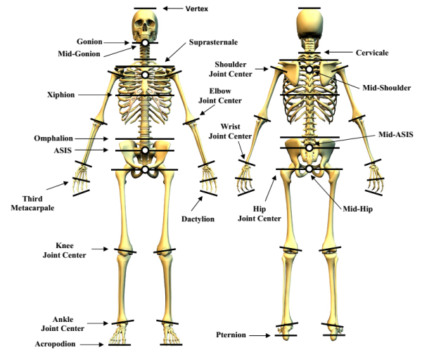
# The segments defined in the Zatsiorsky's model (Zatsiorsky, 2002) adjusted by de Leva (1996) are illustrated in the next figure.
#
#
Figure. Segment definition employed in the anthropometric model of Zatsiorsky and Seluyanov (Zatsiorsky, 2002) adjusted by de Leva (1996). Image from a Motion Analysis Corporation manual.
# In[4]:
BSP_Zmarks = pd.read_csv('https://raw.githubusercontent.com/BMClab/BMC/master/data/BSPlandmarks_ZdeLeva.txt', sep='\t')
display(Latex('\\text{BSP landmarks from Zatsiorsky\'s model adjusted by de Leva (1996):}'))
display(BSP_Zmarks)
# In[5]:
bsp_Zf = pd.read_csv('https://raw.githubusercontent.com/BMClab/BMC/master/data//BSPfemale_ZdeLeva.txt', index_col=0, sep='\t')
display(Latex('\\text{BSP female values from Zatsiorsky\'s model adjusted by de Leva (1996):}'))
display(bsp_Zf)
# In[6]:
bsp_Zm = pd.read_csv('https://raw.githubusercontent.com/BMClab/BMC/master/data/BSPmale_ZdeLeva.txt', index_col=0, sep='\t')
display(Latex('\\text{BSP male values from Zatsiorsky\'s model adjusted by de Leva (1996):}'))
display(bsp_Zm)
# ### Differences between the anthropometric models from Dempster and Zatsiorsky
#
# The anthropometric models from Dempster and Zatsiorsky are different in many aspects; regarding the subjetcs investigated in the studies, Dempster's model is based on the data of 8 cadavers of older male individuals (but two of the individuals were of unknown age) analyzed in the United States. Zatsiorsky's model is based on image scanning of 100 young men and 15 young women, at the time all students of a military school in the former Soviet Union.
#
# The difference between models for some segments is large (see table below): the mass fraction of the thigh segment for Zatsiorsky's model is more than 40% larger than for the Dempster's model, inversely, the trunk segment has about 15% lower mass fraction for Zatisorsky's model. Also, note that some of the segments don't have the same definition in the two models.
# In[7]:
m_D = bsp_D.loc[['Foot', 'Leg', 'Thigh', 'Pelvis', 'Abdomen', 'Thorax', 'Trunk',
'Upper arm', 'Forearm', 'Hand', 'Head neck'], 'Mass']
m_Zf = bsp_Zf.loc[['Foot', 'Shank', 'Thigh', 'Lower trunk', 'Middle trunk', 'Upper trunk',
'Trunk', 'Upper arm', 'Forearm', 'Hand', 'Head'], 'Mass']
m_Zm = bsp_Zm.loc[['Foot', 'Shank', 'Thigh', 'Lower trunk', 'Middle trunk', 'Upper trunk',
'Trunk', 'Upper arm', 'Forearm', 'Hand', 'Head'], 'Mass']
m_D.index = m_Zf.index # because of different names for some segments
display(Latex("\\text{Mass fraction difference (in %) of Zatsiorsky's model w.r.t. Dempster's model}"))
d = pd.DataFrame({'Females': np.around(100 * (m_Zf - m_D) / m_D), \
'Males': np.around(100 * (m_Zm - m_D) / m_D)})
display(d)
# ## Center of mass
#
# See the notebook [Center of Mass and Moment of Inertia](https://nbviewer.jupyter.org/github/BMClab/bmc/blob/master/notebooks/CenterOfMassAndMomentOfInertia.ipynb) for a description of center of mass.
#
# Using the data of the body segment parameters table, the center of mass of a single segment $i$ is (see figure below):
#
# \begin{equation}
# r_{i} = r_{i,p} + \text{bsp[i,cmp]} \cdot (r_{i,d}-r_{i,p})
# \label{}
# \end{equation}
#
# Where $r_{i,p}$ and $\:r_{i,d}$ are the positions of the proximal and distal landmarks used to define the $i$ segment.
# Note that $r$ is a vector and may have more than one dimension. The equation for the center of mass is valid in each direction and the calculations are performed independently in each direction. In addition, there is no need to include the mass of the segment in the equation above; the mass of the segment is used only when there is more than one segment.
#
# For example, given the following coordinates ($x, y$) for the MT2, ankle, knee and hip joints:
# In[8]:
r = np.array([[101.1, 1.3], [84.9, 11.0], [86.4, 54.9], [72.1, 92.8]])/100
display(np.around(r, 3))
# The position of the center of mass of each segment and of the lower limb are:
# In[9]:
M = bsp_D.loc[['Foot', 'Leg', 'Thigh'], 'Mass'].sum()
rcm_foot = r[1] + bsp_D.loc['Foot', 'CM prox']*(r[0]-r[1])
rcm_leg = r[2] + bsp_D.loc['Leg', 'CM prox']*(r[1]-r[2])
rcm_thigh = r[3] + bsp_D.loc['Thigh','CM prox']*(r[2]-r[3])
rcm = (bsp_D.loc['Foot','Mass']*rcm_foot + bsp_D.loc['Leg','Mass']*rcm_leg + \
bsp_D.loc['Thigh','Mass']*rcm_thigh)/M
print('Foot CM: ', np.around(rcm_foot, 3), 'm')
print('Leg CM: ', np.around(rcm_leg, 3), 'm')
print('Thigh CM: ', np.around(rcm_thigh, 3), 'm')
print('Lower limb CM: ', np.around(rcm, 3), 'm')
# And here is a geometric representation of part of these calculations:
# In[10]:
plt.rc('axes', labelsize=14, linewidth=1.5)
plt.rc('xtick', labelsize=14)
plt.rc('ytick', labelsize=14)
plt.rc('lines', markersize=8)
hfig, hax = plt.subplots(1, 1, figsize=(10, 5))
# bones and joints
plt.plot(r[:,0], r[:,1], 'b-')
plt.plot(r[:,0], r[:,1], 'ko', label='joint')
# center of mass of each segment
plt.plot(rcm_foot[0], rcm_foot[1], 'go', label='segment center of mass')
plt.plot(rcm_leg[0], rcm_leg[1], 'go', rcm_thigh[0], rcm_thigh[1], 'go')
# total center of mass
plt.plot(rcm[0], rcm[1], 'ro', label='total center of mass')
hax.legend(frameon=False, loc='upper left', fontsize=12, numpoints=1)
plt.arrow(0, 0, r[3,0], r[3,1], color='b', head_width=0.02, overhang=.5, fc="k", ec="k",
lw=2, length_includes_head=True)
plt.arrow(r[3,0], r[3,1], rcm_thigh[0] - r [3,0], rcm_thigh[1] - r[3,1], head_width=0.02,
overhang=.5, fc="b", ec="b", lw=2, length_includes_head=True)
plt.arrow(0, 0, rcm_thigh[0], rcm_thigh[1], head_width=0.02, overhang=.5, fc="g", ec="g",
lw=2, length_includes_head=True)
plt.text(0.30, .5, '$\mathbf{r}_{thigh,p}$', rotation=38, fontsize=16)
plt.text(0.77, .85, '$bsp_{thigh,cmp}*(\mathbf{r}_{i,d}-\mathbf{r}_{i,p})$',
fontsize=16, color='b')
plt.text(0.15, .05,
'$\mathbf{r}_{thigh,cm}=\mathbf{r}_{i,p}+bsp_{i,cmp}*' +
'(\mathbf{r}_{i,d}-\mathbf{r}_{i,p})$',
rotation=25, fontsize=16, color='g')
hax.set_xlim(0,1.1)
hax.set_ylim(0,1.05)
hax.set_xlabel('x [m]')
hax.set_ylabel('y [m]')
hax.set_title('Determination of center of mass', fontsize=16)
hax.grid()
# ## Moment of inertia
#
# ### Radius of gyration
#
# See the notebook [Center of Mass and Moment of Inertia](https://nbviewer.jupyter.org/github/BMClab/bmc/blob/master/notebooks/CenterOfMassAndMomentOfInertia.ipynb) for a description of moment of inertia and radius of gyration.
#
# The radius of gyration (as a fraction of the segment length) is the quantity that is given in the table of body segment parameters. Because of that, we don't need to sum each element of mass of the segment to calculate its moment of inertia; we just need to take the mass of the segment times the radius or gyration squared.
#
# Using the body segment parameters, the moment of inertia of a single segment $i$ rotating around its own center of mass is (see figure below):
#
# \begin{equation}
# I_{i,cm} = M \cdot \text{bsp[i,mass]} \cdot \left(\text{bsp[i,rgcm]} \cdot ||r_{i,d}-r_{i,p}||\right)^2
# \label{}
# \end{equation}
#
# Where $M$ is the total body mass of the subject and $||r_{i,d}-r_{i,p}||$ is the length of the segment $i$.
#
# For example, the moment of inertia of each segment of the lower limb around each corresponding segment center of mass considering the coordinates (x, y) for the MT2, ankle, knee and hip joints given above are:
# In[11]:
norm = np.linalg.norm
M = 100 # body mass
Icm_foot = M*bsp_D.loc['Foot', 'Mass']*((bsp_D.loc['Foot', 'Rg CM']*norm(r[0]-r[1]))**2)
Icm_leg = M*bsp_D.loc['Leg', 'Mass']*((bsp_D.loc['Leg', 'Rg CM']*norm(r[1]-r[2]))**2)
Icm_thigh = M*bsp_D.loc['Thigh','Mass']*((bsp_D.loc['Thigh','Rg CM']*norm(r[2]-r[3]))**2)
print('Icm foot: ', np.around(Icm_foot, 3), 'kgm2')
print('Icm leg: ', np.around(Icm_leg, 3), 'kgm2')
print('Icm thigh: ', np.around(Icm_thigh, 3), 'kgm2')
# ### Parallel axis theorem
#
# See the notebook [Center of Mass and Moment of Inertia](https://nbviewer.jupyter.org/github/BMClab/bmc/blob/master/notebooks/CenterOfMassAndMomentOfInertia.ipynb) for a description of parallel axis theorem.
#
# For example, using the parallel axis theorem the moment of inertia of the lower limb around its center of mass is:
# In[12]:
Icmll = (Icm_foot + M*bsp_D.loc['Foot', 'Mass']*norm(rcm-rcm_foot )**2 + \
Icm_leg + M*bsp_D.loc['Leg', 'Mass']*norm(rcm-rcm_leg )**2 + \
Icm_thigh + M*bsp_D.loc['Thigh','Mass']*norm(rcm-rcm_thigh)**2)
print('Icm lower limb: ', np.around(Icmll, 3), 'kgm2')
# To calculate the moment of inertia of the lower limb around the hip, we use again the parallel axis theorem:
# In[13]:
Ihipll = (Icm_foot + M*bsp_D.loc['Foot', 'Mass']*norm(r[3]-rcm_foot )**2 + \
Icm_leg + M*bsp_D.loc['Leg', 'Mass']*norm(r[3]-rcm_leg )**2 + \
Icm_thigh + M*bsp_D.loc['Thigh','Mass']*norm(r[3]-rcm_thigh)**2)
print('Ihip lower limb: ', np.around(Ihipll, 3), 'kgm2')
# Note that for the correct use of the parallel axis theorem we have to input the moment of inertia around the center of mass of each body. For example, we CAN NOT calculate the moment of inertia around the hip with the moment of inertia of the entire lower limb:
# In[14]:
# THIS IS WRONG:
I = (Icm_foot + M*bsp_D.loc['Foot', 'Mass']*norm(r[3]-rcm)**2 + \
Icm_leg + M*bsp_D.loc['Leg', 'Mass']*norm(r[3]-rcm)**2 + \
Icm_thigh + M*bsp_D.loc['Thigh','Mass']*norm(r[3]-rcm)**2)
print('Icm lower limb: ', np.around(I, 3), 'kgm2. THIS IS WRONG!')
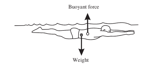
# ## Center of buoyancy
#
# [Center of buoyancy](https://en.wikipedia.org/wiki/Buoyancy) is the center of the volume of water which the submerged part of an object displaces. Center of buoyancy is to center of volume as center of gravity is to center of mass.
#
# For the human body submerged in water, because different parts of the body have different densities, the center of buoyancy is at a different place than the center of gravity, see for example [Yanai and Wilson (2008)](https://onlinelibrary.wiley.com/doi/pdf/10.1002/jst.23).
#
#
Figure. Forces of gravity and buoyancy acting respectively on the center of gravity and center of buoyancy in a submerged human body (figure from Yanai and Wilson (2008)).
# ## Further reading
#
# - [Drill et a. (1964)](http://www.oandplibrary.org/al/1964_01_044.asp) and [Bjørnstrup (1995)](http://citeseerx.ist.psu.edu/viewdoc/summary?doi=10.1.1.21.5223) for a historical overview on the estimation of body segment parameters.
# ## Video lectures on the internet
#
# - [Body segments parameters in Biomechanics](https://youtu.be/8hyPiha-lFU)
# - [Estimating and Visualizing the Inertia of the Human Body with Python](https://youtu.be/H9AK65ZY-Vw)
# ## Problems
#
# 1. Take a picture at the frontal plane of somebody standing on one foot on tiptoes with the arms and the other leg abducted at the horizontal.
# 1. Estimate the body center of mass of this person. Hint: for simplicity, consider the center of mass of each segment to be located at the middle of the segment and measure these positions using a image digitizer, e.g., [WebPlotDigitizer](https://automeris.io/WebPlotDigitizer/).
# 2. If the person is almost standing still, through which part of the body a vertical line through the center of mass should necessarily pass? Have you obtained this result? Comment on possible differences between the expected and obtained results.
#
# 2. Consider the kinematic data from table A.1 of the Winter's book (Winter, 2009) used in problem 2 of the notebook [Angular kinematics in a plane (2D)](http://nbviewer.jupyter.org/github/demotu/BMC/blob/master/notebooks/KinematicsAngular2D.ipynb).
# 1. Calculate the center of mass position for each segment and for the whole body (beware that no data are given for the head and arms segments) using the Dempster's and Zatsiorsky's models.
# 2. Perform these calculations also for the moment of inertia (of each segment and of the whole body around the corresponding centers of mass).
#
# 3. Consider the following positions of markers placed on a leg (described in the laboratory coordinate system with coordinates $x, y, z$ in cm, the $x$ axis points forward and the $y$ axes points upward): lateral malleolus (**lm** = [2.92, 10.10, 18.85]), medial malleolus (**mm** = [2.71, 10.22, 26.52]), fibular head (**fh** = [5.05, 41.90, 15.41]), and medial condyle (**mc** = [8.29, 41.88, 26.52]). Define the ankle joint center as the centroid between the **lm** and **mm** markers and the knee joint center as the centroid between the **fh** and **mc** markers (same data as in problem 1 of the notebook [Rigid-body transformations (3D)](http://nbviewer.ipython.org/github/demotu/BMC/blob/master/notebooks/Transformation3D.ipynb)). Consider that the principal axes of the leg are aligned with the axes of the respective anatomical coordinate system.
# 1. Determine the center of mass position of the leg at the anatomical and laboratory coordinate systems.
# 2. Determine the inertia tensor of the leg for a rotation around its proximal joint and around its center of mass.
# ## References
#
# - Bjørnstrup J (1995) [Estimation of Human Body Segment Parameters - Historical Background](http://citeseerx.ist.psu.edu/viewdoc/summary?doi=10.1.1.21.5223). Technical Report.
# - de Leva P (1996) [Adjustments to Zatsiorsky-Seluyanov's segment inertia parameters](http://ebm.ufabc.edu.br/wp-content/uploads/2013/12/Leva-1996.pdf). Journal of Biomechanics, 29, 9, 1223-1230.
# - Dembia C, Moore JK, Hubbard M (2014) [An object oriented implementation of the Yeadon human inertia model](https://www.ncbi.nlm.nih.gov/pmc/articles/PMC4329601/). F1000Research. 2014;3:223. doi:10.12688/f1000research.5292.2.
# - Drills R, Contini R, Bluestein M (1964) [Body segment parameters: a survey of measurement techniques](http://www.oandplibrary.org/al/1964_01_044.asp). Artificial Limbs, 8, 44-66.
# - Kwon Y-H (1998) [BSP Estimation Methods](http://kwon3d.com/theory/bsp.html).
# - Ruina A, Rudra P (2013) [Introduction to Statics and Dynamics](http://ruina.tam.cornell.edu/Book/index.html). Oxford University Press.
# - Winter DA (2009) [Biomechanics and motor control of human movement](http://books.google.com.br/books?id=_bFHL08IWfwC). 4 ed. Hoboken, EUA: Wiley.
# - Yanai T, Wilson BD (2008) [How does buoyancy influence front-crawl performance?
# Exploring the assumptions](https://onlinelibrary.wiley.com/doi/pdf/10.1002/jst.23). Sports Technol., 1 2–3, 89–99.
# - Zatsiorsky VM (2002) [Kinetics of human motion](http://books.google.com.br/books?id=wp3zt7oF8a0C&lpg=PA571&ots=Kjc17DAl19&dq=ZATSIORSKY%2C%20Vladimir%20M.%20Kinetics%20of%20human%20motion&hl=pt-BR&pg=PP1#v=onepage&q&f=false). Champaign, IL: Human Kinetics.
# - Some of the original works on body segment parameters:
# - Contini R (1972) [Body Segment Parameters, Part II](http://www.oandplibrary.org/al/1972_01_001.asp). Artificial Limbs, 16, 1-19.
# - Dempster WT (1955) [Space requirements of the seated operator: geometrical, kinematic, and mechanical aspects of the body, with special reference to the limbs](http://deepblue.lib.umich.edu/handle/2027.42/4540). WADC Technical Report 55-159, AD-087-892, Wright-Patterson Air Force Base, Ohio.
# - Hanavan EP (1964). [A mathematical model of the human body](http://www.dtic.mil/cgi-bin/GetTRDoc?AD=AD0608463). AMRL-TR-64-102, AD-608-463. Aerospace Medical Research Laboratories, Wright-Patterson Air Force Base, Ohio.