#!/usr/bin/env python
# coding: utf-8
# A Dockerfile that will produce a container with all the dependencies necessary to run this notebook is available [here](https://github.com/AustinRochford/notebooks).
# Clear the `theano` cache before each run to avoid subtle bugs.
# In[1]:
get_ipython().system('rm -rf /home/jovyan/.theano/')
# In[2]:
get_ipython().run_line_magic('matplotlib', 'inline')
# In[3]:
import datetime
from itertools import product
import logging
import pickle
from warnings import filterwarnings
# In[4]:
import arviz as az
from matplotlib import pyplot as plt
from matplotlib.offsetbox import AnchoredText
from matplotlib.ticker import FuncFormatter, StrMethodFormatter
import numpy as np
import pandas as pd
import pymc3 as pm
import scipy as sp
import seaborn as sns
from sklearn.preprocessing import LabelEncoder
from theano import shared, tensor as tt
# In[5]:
# keep theano from complaining about compile locks for small models
(logging.getLogger('theano.gof.compilelock')
.setLevel(logging.CRITICAL))
# silence PyMC3 warnings (there aren't many)
filterwarnings(
'ignore', ".*diverging samples after tuning.*",
module='pymc3'
)
filterwarnings(
'ignore', ".*acceptance probability.*",
module='pymc3'
)
# In[6]:
pct_formatter = StrMethodFormatter('{x:.1%}')
svpct_formatter = ba_formatter = StrMethodFormatter("{x:.3f}")
sns.set(color_codes=True)
# configure pyplot for readability when rendered as a slideshow and projected
plt.rc('figure', figsize=(8, 6))
LABELSIZE = 14
plt.rc('axes', labelsize=LABELSIZE)
plt.rc('axes', titlesize=LABELSIZE)
plt.rc('figure', titlesize=LABELSIZE)
plt.rc('legend', fontsize=LABELSIZE)
plt.rc('xtick', labelsize=LABELSIZE)
plt.rc('ytick', labelsize=LABELSIZE)
# In[7]:
SEED = 54902 # from random.org, for reproducibility
# # Probabilistic Programming for Sports Analytics
#
# ## Bayesian Data Analysis Meetup • April 18, 2019 • New York City
# ## [@AustinRochford](https://twitter.com/AustinRochford)
# ## About Me
#
#  #
# ### Chief Data Scientist @ [Monetate](http://www.monetate.com/) • PyMC3 contributor
#
# ### [@AustinRochford](https://twitter.com/AustinRochford) • [austinrochford.com](http://austinrochford.com) • [github.com/AustinRochford](http://github.com/AustinRochford)
#
# ### [arochford@monetate.com](mailto:arochford@monetate.com) • [austin.rochford@gmail.com](mailto:arochford@monetate.com)
# ## About Monetate
#
#
#
# ### Chief Data Scientist @ [Monetate](http://www.monetate.com/) • PyMC3 contributor
#
# ### [@AustinRochford](https://twitter.com/AustinRochford) • [austinrochford.com](http://austinrochford.com) • [github.com/AustinRochford](http://github.com/AustinRochford)
#
# ### [arochford@monetate.com](mailto:arochford@monetate.com) • [austin.rochford@gmail.com](mailto:arochford@monetate.com)
# ## About Monetate
#
#  #
# * Founded 2008, web optimization and personalization SaaS
# * Observed 5B impressions and $4.1B in revenue during Cyber Week 2017
#
#
#
# * Founded 2008, web optimization and personalization SaaS
# * Observed 5B impressions and $4.1B in revenue during Cyber Week 2017
#
#  # monetate.com/about/careers
#
# ## Agenda
#
# * Sports analytics
# * Heuristics and uncertainty
# * First steps
# * Batting average
# * Save percentage
# * NBA foul calls
# * Future work
# # Sports Analytics
#
#
#
# monetate.com/about/careers
#
# ## Agenda
#
# * Sports analytics
# * Heuristics and uncertainty
# * First steps
# * Batting average
# * Save percentage
# * NBA foul calls
# * Future work
# # Sports Analytics
#
#
#  #
#
#
#
#
#  #
#
#
#
#
#  #
#
#
#
#
#
#
#
#  #
# |
#
#  #
# |
#
#
#
# ## Heuristics and Uncertainty
#
# > The basic blueprint for predicting a player’s upcoming season from his past is the Marcel method, introduced by prominent baseball and hockey analyst Tom Tango back in 2005. It’s a three-step process that
# > 1. starts with a weighted average of a player’s three most recent seasons;
# > 2. regresses that player’s performance toward the league mean, based on games played (we’ll explain why and how in a moment); and
# > 3. applies an age adjustment to account for developing rookies and declining veterans. With regard to the first step, Tango proposes a weighting of 5-4-3, while I prefer a 4-2-1 approach that assumes that every season’s data has twice the predictive power as the season previous.
#
# Vollman, Rob, Awad, Tom, Fyffe, Iain. _Hockey Abstract Presents_ Stat Shot. ECW Press. Kindle Edition.
#
# 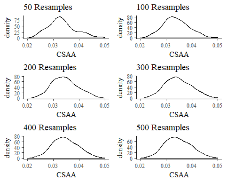 # Bayesian Bagging to Generate Uncertainty Intervals: A Catcher Framing Story
#
# # First Steps
#
# ## Batting Average
# In[8]:
def get_data_url(filename):
return f"https://www.austinrochford.com/resources/sports_precision/{filename}"
# In[9]:
def load_data(filepath, player_col, usecols):
df = pd.read_csv(filepath, usecols=[player_col] + usecols)
return (pd.concat((df[player_col]
.str.split('\\', expand=True)
.rename(columns={0: 'name', 1: 'player_id'}),
df.drop(player_col, axis=1)),
axis=1)
.rename(columns=str.lower)
.groupby(['player_id', 'name'])
.first() # players that switched teams have their entire season stats listed once per team
.reset_index('name'))
# In[10]:
mlb_df = load_data(get_data_url('2018_batting.csv'), 'Name', ['AB', 'H'])
# In[11]:
mlb_df.head()
# In[12]:
batter_df = mlb_df[mlb_df['ab'] > 0]
n_player, _ = batter_df.shape
# [Batting average](https://en.wikipedia.org/wiki/Batting_average_(baseball%29) is the most basic summary of a player's batting performance and is defined as their number of hits divided by their number of at bats. In order to assess the amount of precision that is justified when calculating batting average, we build a hierarchical logistic model. Let $n_i$ be the number of at bats for the $i$-th player and let $y_i$ be their number of hits. Our model is
#
# $$
# \begin{align*}
# \mu_{\eta}
# & \sim N(0, 5^2) \\
# \sigma_{\eta}
# & \sim \textrm{Half-}N(2.5^2) \\
# \eta_i
# & \sim N(\mu, \sigma_{\eta}^2) \\
# \textrm{ba}_i
# & = \textrm{sigm}(\eta_i) \\
# y_i\ |\ n_i
# & \sim \textrm{Binomial}(n_i, \textrm{ba}_i).
# \end{align*}
# $$
#
# We specify this model in [`pymc3`](https://docs.pymc.io/) below using a [non-centered parametrization](https://twiecki.github.io/blog/2017/02/08/bayesian-hierchical-non-centered/).
# In[13]:
def hierarchical_normal(name, shape, μ=None):
if μ is None:
μ = pm.Normal(f"μ_{name}", 0., 5.)
Δ = pm.Normal(f"Δ_{name}", shape=shape)
σ = pm.HalfNormal(f"σ_{name}", 2.5)
return pm.Deterministic(name, μ + Δ * σ)
# In[14]:
with pm.Model() as mlb_model:
η = hierarchical_normal("η", n_player)
ba = pm.Deterministic("ba", pm.math.sigmoid(η))
hits = pm.Binomial("hits", batter_df['ab'], ba, observed=batter_df['h'])
# We proceeed to sample from the model's posterior distribution.
# In[15]:
CHAINS = 3
SEED = 88564 # from random.org, for reproducibility
SAMPLE_KWARGS = {
'draws': 1000,
'tune': 1000,
'chains': CHAINS,
'cores': CHAINS,
'random_seed': list(SEED + np.arange(CHAINS))
}
# In[16]:
with mlb_model:
mlb_trace = pm.sample(**SAMPLE_KWARGS)
# Before drawing conclusions from the posterior samples, we use [`arviz`](https://arviz-devs.github.io/arviz/index.html) to verify that there are no obvious problems with the sampler diagnostics.
# In[17]:
az.plot_energy(mlb_trace);
# In[18]:
(az.rhat(mlb_trace).max().to_array().max())
# First we'll examine the posterior distribution of [Mike Trout](https://www.baseball-reference.com/players/t/troutmi01.shtml)'s batting average.
# ### Mike Trout
# In[19]:
fig, ax = plt.subplots(figsize=(8, 6))
trout_ix = (batter_df.index == 'troutmi01').argmax()
ax.hist(mlb_trace['ba'][:, trout_ix], bins=30, alpha=0.5, lw=0.);
ax.vlines(batter_df['h']
.div(batter_df['ab'])
.loc['troutmi01'],
0, 275,
linestyles='--',
label="Actual batting average");
ax.xaxis.set_major_formatter(ba_formatter);
ax.set_xlabel("Batting average");
ax.set_yticks([]);
ax.set_ylabel("Posterior density");
ax.legend();
ax.set_title("Mike Trout");
# In[20]:
fig
# ### Mike Trout vs. Bryce Harper
# In[21]:
fig, ax = plt.subplots(figsize=(8, 6))
ax.hist(mlb_trace['ba'][:, trout_ix], bins=30, alpha=0.5, lw=0.);
ax.vlines(batter_df['h']
.div(batter_df['ab'])
.loc['troutmi01'],
0, 275,
linestyles='--',
label="Actual batting average");
ax.xaxis.set_major_formatter(ba_formatter);
ax.set_xlabel("Batting average");
ax.set_yticks([]);
ax.set_ylabel("Posterior density");
ax.legend();
ax.set_title("Mike Trout");
harper_ix = (batter_df.index == 'harpebr03').argmax()
ax.hist(mlb_trace['ba'][:, harper_ix], bins=30, alpha=0.5, lw=0.);
ax.vlines(batter_df['h']
.div(batter_df['ab'])
.loc['harpebr03'],
0, 275,
linestyles='--');
ax.xaxis.set_major_formatter(ba_formatter);
ax.set_xlabel("Batting average");
ax.set_yticks([]);
ax.set_ylabel("Posterior density");
ax.legend();
ax.set_title("Mike Trout");
# In[22]:
fig
# In[23]:
fig, ax = plt.subplots(figsize=(8, 8))
ax.set_aspect('equal');
ax.scatter(mlb_trace['ba'][:, harper_ix],
mlb_trace['ba'][:, trout_ix],
alpha=0.25);
BA_RANGE = [0.18, 0.37]
ax.plot(BA_RANGE, BA_RANGE, '--', c='k');
ax.set_xlim(*BA_RANGE);
ax.set_xlabel("Bryce Harper");
ax.set_ylim(*BA_RANGE);
ax.set_ylabel("Mike Trout");
ax.set_title("Posterior Expected Batting Average");
# In[24]:
fig
# In[25]:
(mlb_trace['ba'][:, harper_ix] < mlb_trace['ba'][:, trout_ix]).mean()
# ### Bryce Harper vs. Rhys Hoskins
# In[26]:
fig, ax = plt.subplots(figsize=(8, 8))
ax.set_aspect('equal');
hoskins_ix = (batter_df.index == 'hoskirh01').argmax()
ax.scatter(mlb_trace['ba'][:, harper_ix],
mlb_trace['ba'][:, hoskins_ix],
alpha=0.25);
BA_RANGE = [0.18, 0.37]
ax.plot(BA_RANGE, BA_RANGE, '--', c='k');
ax.set_xlim(*BA_RANGE);
ax.set_xlabel("Bryce Harper");
ax.set_ylim(*BA_RANGE);
ax.set_ylabel("Rhys Hoskins");
ax.set_title("Posterior Expected Batting Average");
# In[27]:
fig
# In[28]:
(mlb_trace['ba'][:, harper_ix] < mlb_trace['ba'][:, hoskins_ix]).mean()
# In[29]:
mlb_df = batter_df.assign(
width_95=sp.stats.iqr(mlb_trace["ba"], axis=0, rng=(2.5, 97.5))
)
# In[30]:
def plot_ci_width(grouped, width):
fig, ax = plt.subplots(figsize=(8, 6))
low = grouped.quantile(0.025)
high = grouped.quantile(0.975)
ax.fill_between(low.index, low, high,
alpha=0.25,
label=f"{width:.0%} interval");
grouped.mean().plot(ax=ax, label="Average")
ax.set_ylabel("Width of 95% credible interval");
ax.legend(loc=0);
return ax
# ### Uncertainty in batting average
# In[31]:
ax = plot_ci_width(mlb_df['width_95'].groupby(mlb_df['ab'].round(-2)), 0.95)
ax.set_xlim(0, mlb_df['ab'].max());
ax.set_xlabel("At bats");
#ax.set_ylim(bottom=0.);
ax.yaxis.set_major_formatter(ba_formatter);
ax.set_title("Batting average");
# In[32]:
ax.figure
# ## Save Percentage
# We apply a similar analysis to save percentage in the NHL. First we load 2018 goaltending data from [Hockey Reference](https://www.hockey-reference.com/leagues/NHL_2018_goalies.html#stats::none).
# In[33]:
nhl_df = load_data(get_data_url('2017_2018_goalies.csv'), 'Player', ['SA', 'SV'])
# In[34]:
nhl_df.head()
# In[35]:
n_goalie, _ = nhl_df.shape
# In[36]:
with pm.Model() as nhl_model:
η = hierarchical_normal("η", n_goalie)
svp = pm.Deterministic("svp", pm.math.sigmoid(η))
saves = pm.Binomial("saves", nhl_df['sa'], svp, observed=nhl_df['sv'])
# In[37]:
with nhl_model:
nhl_trace = pm.sample(nuts_kwargs={'target_accept': 0.9}, **SAMPLE_KWARGS)
# In[38]:
az.plot_energy(nhl_trace);
# In[39]:
az.rhat(nhl_trace).max()
# ### Sergei Bobrovsky
# In[40]:
fig, ax = plt.subplots(figsize=(8, 6))
bobs_ix = (nhl_df.index == 'bobrose01').argmax()
ax.hist(nhl_trace['svp'][:, bobs_ix], bins=30, alpha=0.5, lw=0.);
ax.vlines(nhl_df['sv']
.div(nhl_df['sa'])
.loc['bobrose01'],
0, 325,
linestyles='--',
label="Actual save percentage");
ax.xaxis.set_major_formatter(ba_formatter);
ax.set_xlabel("Save percentage");
ax.set_ylabel("Posterior density");
ax.legend(loc=2);
ax.set_title("Sergei Bobrovsky");
# In[41]:
fig
# ### Uncertainty in save percentage
# In[42]:
nhl_df = nhl_df.assign(
width_95=sp.stats.iqr(nhl_trace["svp"], axis=0, rng=(2.5, 97.5))
)
# In[43]:
ax = plot_ci_width(nhl_df['width_95'].groupby(nhl_df['sa'].round(-2)), 0.95)
ax.set_xlim(0, nhl_df['sa'].max());
ax.set_xlabel("Shots against");
ax.set_ylim(bottom=0.);
ax.yaxis.set_major_formatter(svpct_formatter);
ax.set_title("Save percentage");
# In[44]:
ax.figure
# The code in the following cell converts this notebook to an HTML slideshow powered by [reveal.js](http://lab.hakim.se/reveal-js/).
# In[3]:
get_ipython().run_cell_magic('bash', '', 'jupyter nbconvert \\\n --to=slides \\\n --reveal-prefix=https://cdnjs.cloudflare.com/ajax/libs/reveal.js/3.2.0/ \\\n --output=pp-sports-analytics-part-1 \\\n ./Probabilistic\\ Programming\\ for\\ Sports\\ Analytics.ipynb\n')
# In[ ]:
# Bayesian Bagging to Generate Uncertainty Intervals: A Catcher Framing Story
#
# # First Steps
#
# ## Batting Average
# In[8]:
def get_data_url(filename):
return f"https://www.austinrochford.com/resources/sports_precision/{filename}"
# In[9]:
def load_data(filepath, player_col, usecols):
df = pd.read_csv(filepath, usecols=[player_col] + usecols)
return (pd.concat((df[player_col]
.str.split('\\', expand=True)
.rename(columns={0: 'name', 1: 'player_id'}),
df.drop(player_col, axis=1)),
axis=1)
.rename(columns=str.lower)
.groupby(['player_id', 'name'])
.first() # players that switched teams have their entire season stats listed once per team
.reset_index('name'))
# In[10]:
mlb_df = load_data(get_data_url('2018_batting.csv'), 'Name', ['AB', 'H'])
# In[11]:
mlb_df.head()
# In[12]:
batter_df = mlb_df[mlb_df['ab'] > 0]
n_player, _ = batter_df.shape
# [Batting average](https://en.wikipedia.org/wiki/Batting_average_(baseball%29) is the most basic summary of a player's batting performance and is defined as their number of hits divided by their number of at bats. In order to assess the amount of precision that is justified when calculating batting average, we build a hierarchical logistic model. Let $n_i$ be the number of at bats for the $i$-th player and let $y_i$ be their number of hits. Our model is
#
# $$
# \begin{align*}
# \mu_{\eta}
# & \sim N(0, 5^2) \\
# \sigma_{\eta}
# & \sim \textrm{Half-}N(2.5^2) \\
# \eta_i
# & \sim N(\mu, \sigma_{\eta}^2) \\
# \textrm{ba}_i
# & = \textrm{sigm}(\eta_i) \\
# y_i\ |\ n_i
# & \sim \textrm{Binomial}(n_i, \textrm{ba}_i).
# \end{align*}
# $$
#
# We specify this model in [`pymc3`](https://docs.pymc.io/) below using a [non-centered parametrization](https://twiecki.github.io/blog/2017/02/08/bayesian-hierchical-non-centered/).
# In[13]:
def hierarchical_normal(name, shape, μ=None):
if μ is None:
μ = pm.Normal(f"μ_{name}", 0., 5.)
Δ = pm.Normal(f"Δ_{name}", shape=shape)
σ = pm.HalfNormal(f"σ_{name}", 2.5)
return pm.Deterministic(name, μ + Δ * σ)
# In[14]:
with pm.Model() as mlb_model:
η = hierarchical_normal("η", n_player)
ba = pm.Deterministic("ba", pm.math.sigmoid(η))
hits = pm.Binomial("hits", batter_df['ab'], ba, observed=batter_df['h'])
# We proceeed to sample from the model's posterior distribution.
# In[15]:
CHAINS = 3
SEED = 88564 # from random.org, for reproducibility
SAMPLE_KWARGS = {
'draws': 1000,
'tune': 1000,
'chains': CHAINS,
'cores': CHAINS,
'random_seed': list(SEED + np.arange(CHAINS))
}
# In[16]:
with mlb_model:
mlb_trace = pm.sample(**SAMPLE_KWARGS)
# Before drawing conclusions from the posterior samples, we use [`arviz`](https://arviz-devs.github.io/arviz/index.html) to verify that there are no obvious problems with the sampler diagnostics.
# In[17]:
az.plot_energy(mlb_trace);
# In[18]:
(az.rhat(mlb_trace).max().to_array().max())
# First we'll examine the posterior distribution of [Mike Trout](https://www.baseball-reference.com/players/t/troutmi01.shtml)'s batting average.
# ### Mike Trout
# In[19]:
fig, ax = plt.subplots(figsize=(8, 6))
trout_ix = (batter_df.index == 'troutmi01').argmax()
ax.hist(mlb_trace['ba'][:, trout_ix], bins=30, alpha=0.5, lw=0.);
ax.vlines(batter_df['h']
.div(batter_df['ab'])
.loc['troutmi01'],
0, 275,
linestyles='--',
label="Actual batting average");
ax.xaxis.set_major_formatter(ba_formatter);
ax.set_xlabel("Batting average");
ax.set_yticks([]);
ax.set_ylabel("Posterior density");
ax.legend();
ax.set_title("Mike Trout");
# In[20]:
fig
# ### Mike Trout vs. Bryce Harper
# In[21]:
fig, ax = plt.subplots(figsize=(8, 6))
ax.hist(mlb_trace['ba'][:, trout_ix], bins=30, alpha=0.5, lw=0.);
ax.vlines(batter_df['h']
.div(batter_df['ab'])
.loc['troutmi01'],
0, 275,
linestyles='--',
label="Actual batting average");
ax.xaxis.set_major_formatter(ba_formatter);
ax.set_xlabel("Batting average");
ax.set_yticks([]);
ax.set_ylabel("Posterior density");
ax.legend();
ax.set_title("Mike Trout");
harper_ix = (batter_df.index == 'harpebr03').argmax()
ax.hist(mlb_trace['ba'][:, harper_ix], bins=30, alpha=0.5, lw=0.);
ax.vlines(batter_df['h']
.div(batter_df['ab'])
.loc['harpebr03'],
0, 275,
linestyles='--');
ax.xaxis.set_major_formatter(ba_formatter);
ax.set_xlabel("Batting average");
ax.set_yticks([]);
ax.set_ylabel("Posterior density");
ax.legend();
ax.set_title("Mike Trout");
# In[22]:
fig
# In[23]:
fig, ax = plt.subplots(figsize=(8, 8))
ax.set_aspect('equal');
ax.scatter(mlb_trace['ba'][:, harper_ix],
mlb_trace['ba'][:, trout_ix],
alpha=0.25);
BA_RANGE = [0.18, 0.37]
ax.plot(BA_RANGE, BA_RANGE, '--', c='k');
ax.set_xlim(*BA_RANGE);
ax.set_xlabel("Bryce Harper");
ax.set_ylim(*BA_RANGE);
ax.set_ylabel("Mike Trout");
ax.set_title("Posterior Expected Batting Average");
# In[24]:
fig
# In[25]:
(mlb_trace['ba'][:, harper_ix] < mlb_trace['ba'][:, trout_ix]).mean()
# ### Bryce Harper vs. Rhys Hoskins
# In[26]:
fig, ax = plt.subplots(figsize=(8, 8))
ax.set_aspect('equal');
hoskins_ix = (batter_df.index == 'hoskirh01').argmax()
ax.scatter(mlb_trace['ba'][:, harper_ix],
mlb_trace['ba'][:, hoskins_ix],
alpha=0.25);
BA_RANGE = [0.18, 0.37]
ax.plot(BA_RANGE, BA_RANGE, '--', c='k');
ax.set_xlim(*BA_RANGE);
ax.set_xlabel("Bryce Harper");
ax.set_ylim(*BA_RANGE);
ax.set_ylabel("Rhys Hoskins");
ax.set_title("Posterior Expected Batting Average");
# In[27]:
fig
# In[28]:
(mlb_trace['ba'][:, harper_ix] < mlb_trace['ba'][:, hoskins_ix]).mean()
# In[29]:
mlb_df = batter_df.assign(
width_95=sp.stats.iqr(mlb_trace["ba"], axis=0, rng=(2.5, 97.5))
)
# In[30]:
def plot_ci_width(grouped, width):
fig, ax = plt.subplots(figsize=(8, 6))
low = grouped.quantile(0.025)
high = grouped.quantile(0.975)
ax.fill_between(low.index, low, high,
alpha=0.25,
label=f"{width:.0%} interval");
grouped.mean().plot(ax=ax, label="Average")
ax.set_ylabel("Width of 95% credible interval");
ax.legend(loc=0);
return ax
# ### Uncertainty in batting average
# In[31]:
ax = plot_ci_width(mlb_df['width_95'].groupby(mlb_df['ab'].round(-2)), 0.95)
ax.set_xlim(0, mlb_df['ab'].max());
ax.set_xlabel("At bats");
#ax.set_ylim(bottom=0.);
ax.yaxis.set_major_formatter(ba_formatter);
ax.set_title("Batting average");
# In[32]:
ax.figure
# ## Save Percentage
# We apply a similar analysis to save percentage in the NHL. First we load 2018 goaltending data from [Hockey Reference](https://www.hockey-reference.com/leagues/NHL_2018_goalies.html#stats::none).
# In[33]:
nhl_df = load_data(get_data_url('2017_2018_goalies.csv'), 'Player', ['SA', 'SV'])
# In[34]:
nhl_df.head()
# In[35]:
n_goalie, _ = nhl_df.shape
# In[36]:
with pm.Model() as nhl_model:
η = hierarchical_normal("η", n_goalie)
svp = pm.Deterministic("svp", pm.math.sigmoid(η))
saves = pm.Binomial("saves", nhl_df['sa'], svp, observed=nhl_df['sv'])
# In[37]:
with nhl_model:
nhl_trace = pm.sample(nuts_kwargs={'target_accept': 0.9}, **SAMPLE_KWARGS)
# In[38]:
az.plot_energy(nhl_trace);
# In[39]:
az.rhat(nhl_trace).max()
# ### Sergei Bobrovsky
# In[40]:
fig, ax = plt.subplots(figsize=(8, 6))
bobs_ix = (nhl_df.index == 'bobrose01').argmax()
ax.hist(nhl_trace['svp'][:, bobs_ix], bins=30, alpha=0.5, lw=0.);
ax.vlines(nhl_df['sv']
.div(nhl_df['sa'])
.loc['bobrose01'],
0, 325,
linestyles='--',
label="Actual save percentage");
ax.xaxis.set_major_formatter(ba_formatter);
ax.set_xlabel("Save percentage");
ax.set_ylabel("Posterior density");
ax.legend(loc=2);
ax.set_title("Sergei Bobrovsky");
# In[41]:
fig
# ### Uncertainty in save percentage
# In[42]:
nhl_df = nhl_df.assign(
width_95=sp.stats.iqr(nhl_trace["svp"], axis=0, rng=(2.5, 97.5))
)
# In[43]:
ax = plot_ci_width(nhl_df['width_95'].groupby(nhl_df['sa'].round(-2)), 0.95)
ax.set_xlim(0, nhl_df['sa'].max());
ax.set_xlabel("Shots against");
ax.set_ylim(bottom=0.);
ax.yaxis.set_major_formatter(svpct_formatter);
ax.set_title("Save percentage");
# In[44]:
ax.figure
# The code in the following cell converts this notebook to an HTML slideshow powered by [reveal.js](http://lab.hakim.se/reveal-js/).
# In[3]:
get_ipython().run_cell_magic('bash', '', 'jupyter nbconvert \\\n --to=slides \\\n --reveal-prefix=https://cdnjs.cloudflare.com/ajax/libs/reveal.js/3.2.0/ \\\n --output=pp-sports-analytics-part-1 \\\n ./Probabilistic\\ Programming\\ for\\ Sports\\ Analytics.ipynb\n')
# In[ ]: