Unconstrained Optimization
$\newcommand{\R}{\mathbb{R}}$
$$ \min_{x \in R^n} \;\; f(x) $$$f$ is a convex function
Methods:
- $f$ is continuously differentiable (smooth) $\rightarrow$ gradient descent
- $f$ is twice continuously differentiable $\rightarrow$ GD, Newton, quasi-Newton
- $f$ is quadratic $\rightarrow$ above + conjugate gradient
- $f$ is not differentiable (non-smooth) $\rightarrow$ subgradient method, SGD (today)
Subgradient
$f: \R^n \to \R$, a subgradient of $f$ at $x$ is a vector $g$ satisfying
$$ f(y) \ge f(x) + \langle g, y-x \rangle, \;\; \forall x,y \in \R^n. $$- Does subgradient always exist?
- There could be multiple subgradients of $f$ at $x$.
- When $f$ is convex and differentiable, $g = \nabla f(x)$.
Gradient vs. Subgradient
Gradient: $s = -\nabla f(x)$ is a descent direction, i.e., $\langle \nabla f(x), s \rangle < 0$.
- Stepping into a descent direction decreases $f$ in the first order:
Gradient vs. Subgradient
Subgradient: $s = -g$ is not necessarily descent.
Ex. $f(x,y) = 2|x| + |y|$
At $(x,y) = (1.5,0)$, $g = (2, 1)$, $-g = (-2, -1)$
using PyPlot

n = 200
x = linspace(-4,4,n)
y = linspace(-4,4,n)

xgrid = repmat(x',n,1)
ygrid = repmat(y,1,n)

z = zeros(n,n)
for i in 1:n
    for j in 1:n
        z[i:i,j:j] = 2abs(x[i]) + abs(y[j])
    end
end

cp = plt[:contour](xgrid, ygrid, z, colors="blue", linewidth=2.0)
plt[:clabel](cp, inline=1, fontsize=8)
# xlabel("x")
# ylabel("y")
#tight_layout()

ax = gca()
ax[:spines]["top"][:set_visible](false) # Hide the top edge of the axis
ax[:spines]["right"][:set_visible](false) # Hide the right edge of the axis
ax[:spines]["left"][:set_position]("center") # Move the right axis to the center
ax[:spines]["bottom"][:set_position]("center") # Most the bottom axis to the center
ax[:xaxis][:set_ticks_position]("bottom") # Set the x-ticks to only the bottom
ax[:yaxis][:set_ticks_position]("left") # Set the y-ticks to only the left

arrow(1.5,0,-2,-1,
	head_width=0.1,
	width=0.00015,
	head_length=0.05,
	overhang=0.5,
    head_starts_at_zero="false",
    facecolor="black")
annotate("(1.5,0)", xy=[1.2; 0.1])
annotate("-g", xy=[0.6; -.8])

PyObject <matplotlib.text.Annotation object at 0x31bb4b9d0>
Subdifferential
$$ \partial f(x) := \{g(x) \in \R^n : f(y) \ge f(x) + \langle g(x), y-x\rangle, \forall y \in \R^n \} $$- When $f$ is convex, $\partial f(x)$ is nonempty on every $x\in \R^n$.
- If $f$ is differentiable: $\partial f(x) = \{ \nabla f(x) \}$.
- If $\partial f(x) = \{g(x)\}$, then $f$ is differentiable at $x$ and $g(x) = \nabla f(x)$.
- $\partial f(x)$ is a closed and convex set - If $f$ is Lipschitz continuous, then $\partial f(x)$ is bounded.
Subgradient
Ex. $f(x) = \|x\|_1 = \sum_{i=1}^n |x_i|$
using PyPlot

n = 200
x = linspace(-1,1,n)
y = linspace(-1,1,n)

xgrid = repmat(x',n,1)
ygrid = repmat(y,1,n)

z = zeros(n,n)
for i in 1:n
    for j in 1:n
        z[i:i,j:j] = abs(x[i]) + abs(y[j])
    end
end

fig = figure("pyplot_surfaceplot",figsize=(10,10))
ax = fig[:add_subplot](1,1,1, projection = "3d")
ax[:plot_surface](xgrid, ygrid, z, rstride=2,edgecolors="k", cstride=2, cmap=ColorMap("gray"), alpha=0.8, linewidth=0.25)
xlabel("x")
ylabel("y")

PyObject <matplotlib.text.Text object at 0x32a10e9d0>
where
$$ g_i = \begin{cases} 1 & \text{if } x_i > 0\\ -1 & \text{if } x_i <0\\ [-1,1] & o.w. \end{cases} $$Subgradient Method
Changes to gradient descent:
- Take a step using a subgradient:
2. Keep $x_\text{best}$: since $f(x_{k+1}) \le f(x_k)$ is not guaranteed, $$ \begin{aligned} & \text{if } f(x_{k+1}) \le f_\text{best}, \\ &\qquad x_\text{best} = x_{k+1}, \;\; f_\text{best} = f(x_{k+1}) \end{aligned} $$
3. Stepsize: linesearch is not possible since search dir is not always descent - Constant stepsize: $\alpha_k = c, \forall k$ - Diminishing stepsize: $\alpha_k \to 0$.
Subgradient Method
Assumptions:
- Objective function $f: \R^n \to \R$ is convex
- $f$ is proper: $f(x) > -\infty, \;\forall x$, and $f(x) < \infty$ for some $x$.
- Subgradient is uniformly bounded, i.e., there exists $M>0$ s.t.
- Starting point has distance $D$ to a solution $x^*$, i.e.,
Convergence (1)
We can show that the $x_\text{best}$ until $k$th iteration satisfies: $$ f(x_{k, \text{best}}) - f(x^*) \le \frac{D^2 + M^2 \sum_{i=1}^k \alpha_i^2}{2\sum_{i=1}^k \alpha_i} $$
Constant stepsize $\alpha_i = c$
- If $k= \text{max iter } K$ (fixed), the optimal constant stepsize is $c = \frac{D}{M\sqrt{K}}$
- $f(x_{K, \text{best}}) - f(x^*) \le \frac{DM}{2\sqrt{K}}$
Recall: gradient descent had a faster $O(1/k)$ conv rate
Convergence (2)
$$ f(x_{k, \text{best}}) - f(x^*) \le \frac{D^2 + M^2 \sum_{i=1}^k \alpha_i^2}{2\sum_{i=1}^k \alpha_i} $$- Diminishing stepsize (not square summable)
- $\alpha_k = \frac{D}{M\sqrt{k}}$
- $f(x_{k, \text{best}}) - f(x^*) \le \mathcal O\left( \frac{DM}{2}\frac{\ln k}{\sqrt{k}} \right)$
Convergence (3)
$$ f(x_{k, \text{best}}) - f(x^*) \le \frac{D^2 + M^2 \sum_{i=1}^k \alpha_i^2}{2\sum_{i=1}^k \alpha_i} $$- Diminishing stepsize (square summable)
- $\sum_{k=1}^\infty \alpha_k^2 < \infty$, $\sum_{k=1}^\infty \alpha_k = \infty$, $\alpha_k \to 0$
- e.g. $\alpha_k = \frac{1}{k}$
- $f(x_{k, \text{best}}) - f(x^*) \to 0$
- Can show a (better) conv rate under strong convexity
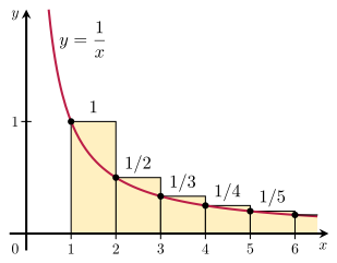
(Side Note) p-Series
$$ \sum_{k=1}^\infty \frac{1}{k^p} $$- $p\le 1$, the series diverges ($p=1$ is called the Harmonic series)
- $p > 1$, the series converges
- Bounds ($p=1$)
- $p=2$ (Euler)
Stochastic (Sub)Gradient Descent (SGD)
Subgradient method + Randomness
Motivation
- Very low per iteration cost
- which may compensate slow convergence
SGD
Consider a objective function with a very large summation:
$$ \min_{x\in X \subset \R^n} \;\; \sum_{i=1}^m \ell(x; D_i) $$where $\ell(\cdot; D_i): \R^n \to \R$ is a convex function.
Convex Loss Functions in Machine Learning
- Square: $\ell(w; x_i, y_i) = (y_i - w^T x_i)^2$ - Hinge: $\ell(w; x_i, y_i) = \max\{ 1 - y_i (\langle w, x_i \rangle), 0 \}$ - Logistic: $\ell(w; x_i, y_i) = \log( 1 + e^{-y_i(\langle w, x_i\rangle)})$ - Huber: $\ell(w; x_i, y_i) = \begin{cases} \frac{1}{2} (y_i-h_w(x_i))^2 & \text{if $|y_i - h_w(x_i)| \le \alpha$} \\ \alpha |y_i - h_w(x_i)| - \frac{1}{2}\alpha^2 & \text{o.w.} \end{cases} $
Full Gradient
The (full) gradient of $f$ will be (assuming $f$ diff'able), $$ \nabla f(x) = \sum_{i=1}^m \; \nabla \ell(x; D_i ) $$
- It will be costly to compute this in each iteration
- It requires to access all data points per iteration (why this is bad?)
Q. Can we avoid this?
Stochastic Subgradient
Consider a stochastic subgradient $G$ of $f$,
$\newcommand{\E}{\mathbb{E}}$
$$ f(y) \ge f(x) + \langle \E[G], y-x \rangle . $$Required property:
- $G$ is unbised
We can consider $G$ as an noisy estimate of $g$, $$ \text{E.g.,}\;\; G = g + v, \;\; g \in \partial f(x), \E[v] = 0 $$
Stochastic Approximation
The usual formulation has
$$ \min_{x \in X}\;\; \tilde f(x) = \frac{1}{m} \sum_{i=1}^m F(x;\xi_i) $$where $m\to\infty$.
This is called Sample Average Approximation (SAA), or Empirical Risk Minimization (ERM)
In data science, what we really want to do is
$$ \min_{x \in X} \;\; f(x) = \E[ F(x;\xi_i) ] = \int_\Xi F(x;\xi) dP(\xi) $$This is called Stochastic Approximation (SA) or Risk Minimization
SGD Assumptions
$$ \min_{x \in X} \;\; f(x) = \E[ F(x;\xi_i) ] = \int_\Xi F(x;\xi) dP(\xi) $$Assumptions:
- $F(\cdot;\xi)$ is convex for each $\xi \in \Xi$. This implies that $f(\cdot)$is convex.
- We can generate i.i.d. samples $\xi_1,\dots,\xi_m$ of the random variable $\xi$.
- $X$ is a nonempty compact convex set
- $f$ is proper
Two constants:
- $\E[ \|G(x,\xi)\|_2^2 ] \le M^2, \;\; \forall x$
- $D = \max_{x\in X} \|x-x_0\|_2$
Classical SGD
$$ x_{k+1} = \text{proj}_{X} (x_k - \alpha_k G(x_k, \xi_k)) $$$f$ is $c$-strongly convex, and stepsize $\alpha_k = \frac{\theta}{k}$ with $\theta > \frac{1}{2c}$,
- $\mathbb E [ \|x_k - x^*\|_2^2 ] \le \frac{1}{k} \max\left\{\frac{\theta^2M^2}{2c\theta-1}, \|x_0-x^*\|_2^2\right\}$
$f$ is diff'able and $\nabla f$ is $L$-Lipschitz continuous, and $x^* \in \text{int}\, X$,
- $\mathbb E [ f(x_k) - f(x^*) ] \le \frac{L}{2k} \max\left\{\frac{\theta^2M^2}{2c\theta-1}, \|x_0-x^*\|_2^2\right\}$
Classical SGD: Issues
The convergence is sensitive to
- $c>0$, i.e. $f$ is strongly convex
- the correctness of the value of $c$
Ex. $f(x) = x^2/10$, $G(x,\xi) = \nabla f(x)$ (no noise), $X = [-1,1]$
- What is the strong convexity constant $c$ of $f(x)$?
Ex. $f(x) = x^2/10$, $G(x,\xi) = \nabla f(x)$ (no noise), $X = [-1,1]$
- Consider that we've chosen $c=1$, $\theta =1 > 1/(2c)$ and $x_1=1$ $\;\Rightarrow\;$ $\alpha_k = 1/k$
With $k=10^9$, we still have $x_k > 0.015$
Robust SGD
Differences to the classical SGD:
- $f$ doesn't have to be strongly convex
- Make a weighted average of iterates (from iterations $s$ to $k$)
- $ D = \max_{x\in X} \|x-x_1\| $
Robust SGD: Convergence
Constant stepsize $\alpha_k = \frac{D}{M\sqrt{K}}$, $$ \E[ f(\tilde x_s^K) - f(x^*) ] \le \frac{DM}{\sqrt{K}} \left[ \frac{2K}{K-s+1} + \frac{1}{2} \right] $$
Diminishing stepsize $\alpha_k = \frac{\theta D}{M\sqrt{k}}$ for any $\theta>0$, $$ \E[ f(\tilde x_s^k) - f(x^*) ] \le \frac{DM}{\sqrt{k}} \left[ \frac{2}{\theta} \left( \frac{k}{k-s+1} \right) + \frac{\theta}{2} \sqrt{\frac{k}{s}} \right] $$
$s = \lceil rk \rceil$, $r \in (0,1)$: $$ \E[ f(\tilde x_s^k) - f(x^*) ] \le \frac{DM}{\sqrt{k}} \left[ \frac{2}{\theta} \left( \frac{1}{1-r} \right) + \frac{\theta}{2} \sqrt{r} \right] $$
Exercises (Ch 10)
For a convex function $f: \R^n \to \R$, show that its subdifferential $\partial f(x)$ is a convex set. (Bonus) Show also that $\partial f(x)$ is closed.
Suppose that $f:\R^n \to \R$ is convex and Lipschitz continuous (with a constant $L>0$). Show that its subgradients are bounded in norm.
Implement the SGD algorithm to solve the SVM (primal form without intercept)
where $x_i \in \R^n$ and $y_i \in \{-1,+1\}$ for $i=1,\dots,m$, and $\lambda>0$. Train the SVM on 60000 training data from the MNIST data set (use the MNIST Julia package and traindata()). Report the prediction accuracy of the trained SVM, on the test data set of 10000 samples not used for training (use testdata()). In SVM, we predict the label of a given input point $x\in\R^n$ as $+1$ if $\langle w^*, x \rangle > 0$, or $-1$ if $\langle w^*, x \rangle < 0$.
- Normalize the data dividing each pixel intensity values by the max. value 255.
- Try both classical and robust stepsize choices, for different values, e.g. $\lambda \in \{1e-3, 1e-4, 1e-5\}$